Quantcast
Channel: ScienceBits - global warming
Viewing all 33 articles
Browse latest View live

The Critique of Knud Jahnke and a New Meteor Exposure Age Analysis

0
0
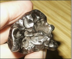
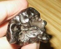
An Iron meteorite, a large sample of which can be used to reconstruct the past cosmic ray flux variations. The reconstructed signal reveals a 145 Myr periodicity shown below. This particular one is part of the Sikhote Alin meteorite that fell over Siberia in the middle of the 20th century, it broke off its parent body about 300 Million years ago.
Last year, a critique by Knud Jahnke appeared on the astro-ph preprint arXiv, in it, my meteoritic-based reconstruction of the cosmic ray flux was heavily criticized. Below, I elaborate on why this criticism is invalid. I also describe a better statistical analysis, one which unequivocally demonstrates that a 143 Myr periodicity does indeed exist in the meteoritic data.

If you landed on this page by accident (i.e., it appears somewhat out of context), I would suggest first reading my description on the spiral arm → cosmic ray → climate link, and the cosmic ray flux signature in the iron meteorites.

General Remarks on Jahnke's critique

The manuscript by Jahnke (which was not accepted for publication by A&A) is an attempt to repeat my previous analyses (e.g., PRL and New Astronomy papers linked from here). Although Jahnke raises a few interesting aspects, his analysis suffers from several acute problems, because of which he obtains his negative result, that is, that there is no statistically significant periodicity in the data and that there is no evidence for cosmic ray flux variability.

By far, the most notable problem is that Jahnke's analysis does not consider the measurement errors. In his analysis, poorly dated meteorites were given the same weight as those with better exposure age determinations. As I show below, this has a grave effect on the signal to noise ratio (S/N) and consequently, on the statistical significance of any result he obtains.

I begin by summarizing the few benign points considered by Jahnke. Then I describe at length the main faults in his analysis, and follow by carrying out a more suitable statistical analysis based on the Rayleigh spectrum method and show that a periodic signal of 145 Myr is present in the data, at a statistically significant confidence level, even if one considers the more stringent grouping chosen by Jahnke.

In the appendix I describe at length why the statistical tool I employ here is better than that used by Jahnke (at least for the type of signals we are looking for in the data) or in fact by myself in the previous analyses. Moreover, the calculation described in the appendix quantifies the S/N degradation brought about by considering poorly dated meteorites, as Jahnke did. This quantitatively shows why his analysis could not have obtained any signal at a statistically significant level.

Simply said, the Jahnke's analysis literally introduces more noise than it does a signal and its null result is basically meaningless.

Detailed Comments


Some benign remarks

  • Since I am not a meteoriticist, I have no way of judging whether all iron meteorites of a single classification group (according to the old or the recent classification) originated from the same parent body, nor whether they broke off at the same event. Thus, it is better in this respect to be more conservative. That is, as Jahnke points out, once recent claims that several iron groups should be grouped together were published, whether they are correct or not, we should consider the more conservative point of view to reduce the possibility that clustering is the result of single events producing multiple meteorites. Nevertheless, from the fact that we have some cases where the exposure ages of many meteorites span a long time range (a few 108yr), it is clear that at least some meteorites of the same iron group classification do not originate from the same meteoritic break up event.

  • As Jahnke points out, the K-S analysis does indeed have a bias, with a higher sensitivity in the center. Such that choosing a phase insensitive statistic is not a bad idea at all. However, as I show below, the analysis done by Jahnke is actually a degradation of the analysis previously done by myself for other reasons. Moreover, the insinuation that I tuned the phase of the K-S to artificially get a better significance has no place. The phase used in the K-S is the phase of the data obtained if the zero-point for the folding is today. That is, there was no tuning in this respect and it should have been checked by Jahnke before making these insinuations.

Critical Points

  • The main difference between the analyses of Jahnke and my previous analysis, is not any of those mentioned by Jahnke. Instead, the main difference is that Jahnke considered meteorites which have very poor error determination. As I show in the appendix, this considerably degrades the signal to noise ratio (S/N). This can be easily seen. If one adds a meteorite which is not expected to contribute any signal (because its phase in the periodicity is effectively unknown due to the error), then the noise is increased without increasing the signal, thereby decreasing the S/N. This will in turn degrade the statistical significance of any positive result. For example, it degrades a signal significant at the 99% level to the notably less significant 90% level. In my previous analysis, I simply discarded meteorites with a quoted error of 100 Myr or more (which actually corresponds to about 70 Myr or more, since Vosage & Feldman overestimated their errors, as can be seen once the potassium ages are compared with other exposure ages). In the present analysis, I simply weigh them according to their expected contribution to the signal.

  • Although the Hierarchical clustering method I employed in the previous analysis is not ideal, it has one major advantage over the "up" or "down" methods devised by Jahnke. That is, Jahnke's method introduces a systematic error in the age of the clustered meteorites. This can be seen by comparing the meteor "clusters" which were assigned different ages according to the direction of the clustering. In all these instances of a different assigned age, the "up" clustering gave an exposure ages which was typically 40 Myr higher than in the "down" case. Clearly, it is unacceptable to have a 1/6 of the meteorites with such a large systematic error. That is to say, the hierarchical method is not ideal, but the modification suggested by Jahnke is even worse. The systematic errors will degrade the signal.

  • Instead of degrading the Hierarchical method as Jahnke did, I introduce below a method which does not suffer from the above problems which arise when clustering the meteorites, though it does consider the possibility that meteorites of the same iron group could arise from the same breakup event. The method also has the advantage that it can straightforwardly be expanded to analyze the error distribution, and independently show that the error include the same 145 Myr cycle.

Re-analysis using the Rayleigh Periodogram

In his analysis, Jahnke introduced several modifications (whether legitimate, such as being more conservative with the meteoritic grouping, or illegitimate, such as carelessly using poorly dated meteorites) which reduced the S/N. Thus, it is worthwhile to see whether another statistical method exists which is better suited to answer the question of whether the clustering is real or not.

The method described in this section is based on the Rayleigh periodogram analysis. It has various advantages and disadvantages relative to the K-S, and its Kuiper statistic cousin.

I begin by describing the method. I then extend it to the analysis of the distribution of errors, and describe its statistically significant results for a 145 Myr signal in the meteoritic data. In the appendix, I compare the method to the Kuiper statistic and show that at least for the type of signals we expect to see in the data, it is a much stronger tool.

The Rayleigh Analysis

The Rayleigh analysis (RA) method is a statistical tool useful for establishing periodic deviations from the uniform occurrence of discrete events. As shown in the appendix, the RA method is better suited for this type of analysis than the Kolmogorov-Smirnov or its Kuiper deviate. This is because the statistical significance obtained for sinusoidal deviations, which are of the kind we are searching here, is notably higher than the significance obtained in the K-S or Kuiper statistic. This is not to say that the RA is better in general. There are many cases where K-S and Kuiper statistics are better suited. For example, they are more appropriate when analyzing deviations from a given nonuniform distribution or finding non-periodic deviations.

The essence of the RA method is finding statistical deviations from a 2D random walk generated by the set of random events. For comparison, the K-S and Kuiper statistics rely on deviations between the observed cumulative distribution of the random events and that of the given distribution. In essence, they are 1D random walks with some constraints.

More specifically, for each period tested by the RA method, the discrete events are assigned phases corresponding to their occurrence within the given period $  p $. A 2D random walk can then be constructed based on the phases, where a step is taken in the direction of $  \cos(\phi_i) {{{\hat{\bf e}}_1}} + \sin(\phi_i) {{\hat{\bf e}}_2} $ where $  {{\hat{\bf e}}_1} $ and $  {{\hat{\bf e}}_2} $ are the two directions of the random walk, and the phase is $  \phi_i = 2 \pi t_i / p $. This walk essentially addresses the question of whether the phases are uniformly distributed or whether concentrated around a certain preferred phase.

If, for example, the events are assigned constant weights, the sum of the walk can be described by the vector
$$ 
{\bf R}(p) = {1\over \sqrt{N}} \left( \sum_i \cos \left( 2 \pi t_i \over p\right) {{\hat{\bf e}}_1} + \sum_i \sin  \left( 2 \pi t_i \over p \right) {{\hat{\bf e}}_2} \right).
$$
If the events exhibit no periodicity $ p $, then the walk should be a random walk. The vector sum R(p) should be 0 on average, and the probability that the power PRR(p)2, also called the Rayleigh power, will be larger than a value a is given by (e.g., Bai, ApJ, 397:584, 1992):
$$ {\mathrm{Prob}} \left( P_R > a \right) = \exp (-a).
$$
If a signal is present in the data, the phases will be aligned if the data points are folded over the period present in the data, and a large PR will be obtained.

Note that this probability is for a given frequency. If we are studying a range of frequencies, then we should increase the probability according to the effective number of frequencies we have. For example, with a 1/1000 Myr-1 resolution (because the data spans about 1000 Myr), we have ~6 independent frequencies between 100 and 250 Myr (the range taken by Jahnke), each one could randomly yield a large value.

The analysis is more complicated because of two important reasons irrespective of the actual method employed (whether K-S, Kuiper or Rayleigh).

First, the meteorites do not have the same weight. Some meteorites, for example, are poorly dated. If they have an error larger than the half the period, then their phase in the Rayleigh analysis will be totally random. Clearly, such "measurements" will only add noise but no real signal, thereby decreasing the SNR (as was done by Jahnke).

Second, meteorites of the same Iron group classification and similar ages are most likely products of the same parent objects which crumbled in the same event (or related events). This implies that not all clustering should be attributed to cosmic ray flux variations.

We shall now discuss both.

Effect of meteoritic age error

If a meteor is poorly dated, it is less likely to appear in the right phase to give the right signal (irrespective of the analysis). In the limit of a large error, it will contribute no signal but will increase the noise. It is therefore wise not to attribute the same weight to all meteorites.

In the Rayleigh analysis, a gaussian distribution for the phases implies that a meteorite is only expected to contribute with a reduced weight of $ w_i = \exp \left( - {2 \pi^2 \sigma^2 / p^2} \right) $. This is obtained after integrating the sine and cosine functions with a gaussian distribution. Thus, a more appropriate form for the power PR(p) is actually:
$$ P_R(p) = {1 \over \sum_i w_i} \left[ \left( \sum_i \cos \left( 2 \pi t_i \over p\right)  w_i \right)^2 + \left( \sum_i \sin  \left( 2 \pi t_i \over p \right) w_i \right)^2 \right].
$$
That is, poorly dated meteorites contribute very little, as they are assigned their actual weight corresponding to their actual contribution towards a signal.

Note that the errors quoted by Vosage et al., are larger than the actual errors. This can be seen if the Potassium age determinations are compared with the other independent exposure age methods (such as using 10Be). Once this is done using the data of Lavielle et al. (EPSL, 170:93, 1999), while remembering the systematic correction necessary for the methods employing short lived isotopes, one obtains that the typical error between the Potassium age determinations and the other methods is about 70% of the quoted error of the Vosage et al. data (The error contribution from the other methods is expected to be small according to the quoted errors they have).

Meteoritic multiplicity

As mentioned numerous times before, some of the clustering could be due to the breakup of a single parent body in one or a few related events. To avoid this problem, it was first suggested in my first analysis to cleanup the data by merging together meteorites of the same iron group classification. As pointed out by Jahnke, this does not come without its problems. Moreover, the cleanup method suggested by Jahnke has even worse problem, as it introduces an unacceptable systematic error in the ages.

The Rayleigh periodogram offers a straightforward extension which does not introduce the systematic errors or the ambiguity of knowing to which cluster a meteorite should be clustered.

Instead of clustering the meteorites together, they can be analyzed separately, with the following two modifications.

First, since meteorites with the same Iron group classifications and a small age separation (e.g.,
Using this modification, we don't increase the statistical weight of a single breakup cluster, nor do we add systematic errors by accidentally merging wrong meteorites. However, the statistical analysis is more complicated and we cannot use the above equation for Prob(PR>a). We will use instead a Monte Carlo simulation.

The modified Rayleigh periodogram and the related Errorgram

Following the above points, I carried out a modified Rayleigh analysis, with a variable weight (assigning a weight according to the error, and then limiting the total weight for each cluster, based on the recent, more stringent, Iron classification).

To estimate the statistical significance, I did a Monte Carlo simulation. Meteoritic break up events were randomly chosen between 100 and 900 Myr, and then smeared with a 200 Myr gaussian distribution to avoid edge effects. Each meteorite was assigned an error from those actually measured. A group of meteorites was simulated as a number of breakup events according to the width of the distribution and calculated as below. The ages of meteorites comprising each breakup event are chosen as the breakup event plus a random error realized using the assigned error of the given meteorite.

The actual number of events a group comprises is calculated as above: total range/100 Myr. If the number is smaller than 1, then 1 group is taken. If larger than one, the number of events is taken as the truncated integer of the obtained number with a probability of one minus the faction obtained. In the other cases, the higher integer is taken as the number of groups. (For example, in the example mentioned above, the 2.9 groups were chosen as 3 events in 90% of the time, and 2 events in 10% of the time).

The Rayleigh periodogram and the variable error permit yet another analysis. Because the errors are not fixed, they too can independently contain a clustering signal.

We define an error vector E as $ {\bf E} = E_1 {{\hat{\bf e}}_1} + E_2 {{\hat{\bf e}}_2} $ with:
$$ E_1(p) = {1\over \sqrt{N}} \left( \sum_i  \sigma_i \cos \left( 2 \pi t_i \over p\right) - {1\over N} \sum_i \sigma_i \sum_i \cos  \left( 2 \pi t_i \over p \right)  \right) $$
$$E_2(p) = {1\over \sqrt{N}} \left( \sum_i  \sigma_i \sin \left( 2 \pi t_i \over p\right) - {1\over N} \sum_i \sigma_i \sum_i \sin  \left( 2 \pi t_i \over p \right)  \right) , $$
where σi is the error on measurement ti. And its power can be defined as $  P_E = E_1^2 + E_2^2 $.

Clearly, if there is no real clustering in the data, then the errors $ \sigma_i $ are not expected to be correlated with ti, in which case $ \sum_i \sigma_i \cos() \rightarrow (\sum_i \sigma_i) (\sum_i \cos())/N $, and E1→ 0 and similarly E2→ 0, even if there is a notably large R. In other words, if a large R is obtained as a statistical fluke, there is no reason a priori for a large E to arise, since there is no reason for the fluke to arrange the errors as well.

However, if the signal in PR(p) is real and not coincidental, we expect a large PE(p) as well. This is because we expect the ages with larger errors to exhibit less clustering around the phase of maximum R, since it is easier for poorly dated meteorites to stray off the preferred phase. We therefore expect E to be in opposite direction of R. This implies that having a large E can be used as an independent indicator to show that the data has a real correlation. Moreover, for consistency, we can also calculate the angle cosine μ between the vectors, which should be ~ -1 if the signal is real:
$$ \mu = {{\bf E} \cdot  {\bf R} \over |{\bf E}| | {\bf R}|}.
$$
since the error size and the clustering are expected to be inversely correlated for a real signal.

Results of the Rayleigh analysis

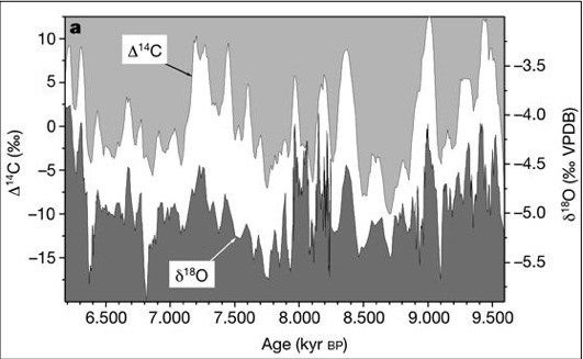
I now proceed to perform the Rayleigh analysis using the stricter grouping suggested by Jahnke.

The Rayleigh power spectrum PR(p), the independent error spectrum PE(p) and the angle between the R and E vectors were calculated as a function of frequency. The results are depicted in the figure.

[collapse title="Power Spectra"]
From bottom to top: The two independent power spectra—the Rayleigh power PR and the independent error spectrum PE. Except for the coincidence of the spectra at a frequency of f ~ 7/1000 Myr-1, the two power spectra do not correlate. Note also that the probability to get a peak with a given amplitude falls exponentially with the amplitude. The middle panel depicts the combined spectrum, showing a remarkable peak at f ~ 7 /1000 Myr-1. The top panel depicts the angle between R and E. For a real signal, not only do we expect to see large PR and PE, but this angle is expected to be of order 180°, and indeed it is. [/collapse] The first point evident from the figure is that PR(f) has a prominent peak at f ~ 7 /1000 Myr-1. The rough estimate for the probability to obtain such a peak between 1/250 Myr-1 and 1/100 Myr-1 (the range used by Jahnke) is 6xexp(-5.5)≅2.5% (6 is the number of independent frequencies, assuming the meteoritic ages span about 1000 Myr). A Monte Carlo simulation (as described above) gives a more reliable estimate, which is actually 6%. That is, there is a 6% chance that a random set of meteorites (even if they have internal multiplicities from breakups), would yield as large a PR as observed.

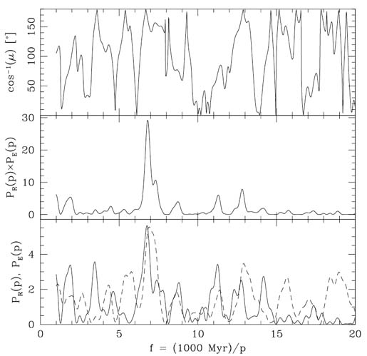
The results of the appendix also explain why the analysis performed by Jahnke could not yield any signal. Degrading the 6% statistical significance any further by letting poorly dated meteorites deteriorate the S/N, or by using the Kuiper statistic with its lower statistical efficiency (relative to the Rayleigh analysis, for this type of a signal), is evidently more than sufficient to remove any trace of the 145 Myr periodicity.

But this is not all. Besides PR there is also the independent PE signal. The Monte Carlo simulation yields a probability of 3.7% to obtain the signal in the error distribution. The combined probability obtained in the Monte Carlo simulation is 0.2% (since it is roughly the product for the probabilities of both spectra, it indicates that the signals are indeed independent).

Last, for consistency, we see that the angle between R and E is around 180°. That is, the vectors point in opposite directions as predicted. Clearly, the 145 Myr signal is present in the data at high statistical significance.

We can refine the test and ask ourselves, what is the probability that a meteoritic exposure age signal will be present in the data which agrees with the periodicity found in ice-age epochs on Earth, that is, with a period of 145 ± 7 Myr. The probabilities for this to occur are 1.0%, 0.6% and 0.06% respectively. Clearly, it would be shear coincidence for the meteoritic exposure ages to happen to (a) exhibit a periodicity in their their exposure ages (b) independently agree in their error distribution (c) agree in the phase between the errors and clustering, (d) and happens to agree with the climatic periodicity! Note also that this doesn't even take into account the fact that the phase of the 145 Myr period in the meteoritic data is in agreement with the phase of the ice-age epochs (which would contribute yet another factor of 5 in the (im)probability estimate).

Summary

I have shown above that the analysis of Jahnke is critically flawed by considering poorly dated meteorites. As I demonstrate in the appendix, this can easily reduce a 1% significant peak to the 10% level. This is the main reason why the 145 Myr peak disappeared from Jahnke's analysis, not the fact that he was more stringent in the clustering he used. As for the two new clustering methods introduced by him, the methods give rise to unacceptable systematic errors and should therefore not be used.

In the new method described above, based on the Rayleigh analysis, no re-clustering is assumed, only a reduction of the meteoritic weights. This has the advantage of introducing no systematic error and lacks the ambiguity present when clustering a large group of meteorites spread over a long period.

Moreover, the Rayleigh analysis appears to be a better method for the type of signals we are testing for (see also Leahy et al., ApJ, 272:256, 1983, who compares the Rayleigh analysis to epoch folding and reach similar conclusions). Once we use a method which is expected to yield a better S/N, we recover the 145 Myr periodicity, with a high confidence level, even if we keep ourselves to a much more stringent data set, as restricted by Jahnke.

It is also worthwhile noting that the periodicity found in the meteoritic exposure ages is not unrelated to other signals, which have consistently the same period and phase.

In particular, the cosmic ray flux is predicted, using purely astronomical data, to vary at roughly the same period (135±25 Myr) and phase. Thus, the fact that a signal is present should not be surprising at all. On the contrary, it would have been a great surprise if no signal would have been observed in the meteorites!

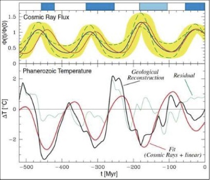
Since cosmic rays are suspected as being a climate driver (with the first suggestion by Ney, already in 1959!), it is also no surprise that various sedimentational and independently geochemical reconstructions of the terrestrial climate reveal climate variations with the same period and phase as that seen in the exposure ages of meteorites.

[collapsed title="Appendix: Rayleigh Analysis and Kuiper statistics comparison"]

Comparison between the Rayleigh Analysis and Kuiper statistics for finding a periodic signal

Above, I presented a statistical analysis based on the Rayleigh periodogram. The question arises, why is this analysis better than the Kuiper analysis (which is the modified K-S analysis used by Jahnke). The answer is that in general, it does not have to be the case, but it certainly is for the type of signals we are looking for. In particular, the K-S and Kuiper analyses, are better suited for finding deviations from a non-uniform distribution and from non-periodic distribution.

The aim of the statistical analyses introduced, either by Jahnke or by myself, is to estimate the probability with which one can rule out the null hypothesis, that the meteorites are distributed homogeneously.

To see the type of statistical significances the methods can yield, we will look at a simple, yet realistic distribution for the ages, and calculate the significances with which the above null hypothesis can be ruled out.

Lets assume that the signal in the data has a probability distribution function of
$$ 
P(t)= {1\over \Delta T} \left[1+\alpha \sin \left(2 \pi t \over p_0\right)\right] 
$$
where ΔT ~ 900 Myr is the total interval over which we have meteorites.

If we have N measurements with the above distribution, the normalized Rayleigh amplitude will be:
$$ 
  {\bf R}(p) = {1\over \sqrt{N}} \left( \sum_i^N \cos \left( 2 \pi t_i \over p\right) {{\hat{\bf e}}_1} + \sum_i^N \sin  \left( 2 \pi t_i \over p \right) {{\hat{\bf e}}_2} \right)
$$
We are interested in the expected signal in the large N limit. Thus, we can approximate the sum with an integral $ \sum_i \rightarrow N \int P(t) dt $. Thus,
$$ 
  {\bf R}(p) = {\sqrt{N} \over \Delta T } \int \left[1+\alpha \sin \left(2 \pi t \over p_0\right)\right]  \left( \cos \left( 2 \pi t_i \over p\right) {{\hat{\bf e}}_1} + \sin  \left( 2 \pi t_i \over p \right) {{\hat{\bf e}}_2} \right)
$$
We are also interested in the peak amplitude, obtained when p = p0. Also, to first approximation, we have that $ \overline{\sin} \approx 0 $ and $ \overline{\sin \cos} \approx 0 $, while $ \overline{\sin^2} \approx 1/2 $. Hence, we find:
$$ 
 {\bf R}(p_0) = {\sqrt{N} \over \Delta T } \Delta T {\alpha \over 2} {{\hat{\bf e}}_2} = {\sqrt{N} \alpha \over 2} {{\hat{\bf e}}_2}.
$$
We are interested in the power, which is:
$$ 
 P_R = R^2(p_0) = { N \alpha^2 \over 4}.
$$
This should be compared with the null hypothesis. If the events are random, then we expect $ \overline{R} = 0 $. The probability that R2 will be larger than a value a is given by
$$ 
{\mathrm{Prob}} \left( P_R > a \right) = \exp (-a)
$$
Thus, the probability that random events will produce a signal as significant as that of a real sinusoidal signal is:
$$ 
{\mathrm{Prob}} \left( P_R > a_{signal} \right) = \exp \left(- {N \alpha^2 \over 4} \right)
$$
If we are interested in 1% probability, we find that the number of events we need is roughly Nmin≅18/α2. (i.e., 18 measurements for α=1 or 72 for α=1/2).

In the case of the Kuiper statistics, we first need to calculate the largest displacement between the cumulative distribution and the homogeneous distribution.

Given the above probability distribution function, folded between 0 and p0, the cumulative function normalized to p0=1 is:
$$ 
   {\mathrm{Prob}} (t>\tau) = \tau - \left( {\alpha \over 2 } \left[ \cos\left( {2 \pi \tau} + \phi_0 \right)  - \cos\left( \phi_0 \right) \right]  \right)  
$$
While for the homogeneous case it is:
$$ 
   {\mathrm{Prob}}(t>\tau) = {\tau }  
$$
The maximum distance above plus the maximum distance below the homogeneous distribution is independent of $ \phi_0 $ and gives:
$$ 
 V = {\alpha \over \pi}
$$
According to the numerical recipes book, the probability to get a fluctuation this large is given by:
$$ 
{\mathrm{Prob}}(>V) = Q_{KP} \left( \left[ \sqrt{N} + 0.155 +0.24/\sqrt{N} \right]V\right) 
$$
where
$$ 
Q_{KP} (\lambda) \equiv 2 \sum_{j=1}^\infty (4j^2 \lambda^2 - 1)\exp(-2j^2\lambda^2) 
$$
With this function, one can calculate the required N to reach a certain accuracy. If we are interested in a 1% goal, and α≅1, we require about 37 measurements. For α≅1/2, we required 153 points.

Thus, for this distribution function, the Rayleigh analysis requires half as many points to reach the same statistical significance. Conversely, for the same number of points, the Kuiper statistic will result with a less significant result for the type of probability distribution function we are interested in. For example, if α≅0.7, 40 points are required to reach a 1% significance with the Rayleigh statistic. The same 40 points, would result with a 28% significance (which is insignificant!) with the Kuiper statistic.

[/collapse] [collapsed title="Appendix B: Degradation by poorly dated meteorites"] The above results also explains why adding noisy points heavily degrades the statistical significance. Suppose we double the number of points, by adding noisy points that have no correlation with the signal. In such a case, we double N, but decrease α by a factor of 2. Since the significance is a function of Nα2, the significance will deteriorate. For example, if we have about 40 points with α≅0.7, the significance will deteriorate from 1% to 10%. It is therefore important not to include in the analysis points with poor error determinations.

[/collapse]

More online Material


ContentType:


Comments on nature's "A cosmic connection"

0
0
Last week, a report by Jeff Kanipe appeared in nature. In it, Kanipe explains the solar → cosmic-ray → climate connection, and the planned CLOUD experiment in CERN, expected to finally resolve the issue. Given that my work is mentioned in the review, I through I should mention a few relevant points.
  • Other galactic/climate mechanisms: Kanipe mentions the work of Shapely, in 1921, who speculated that passing through a dense molecular cloud would make earth colder. Other ideas include accretion of interstellar dust, which would block sun light, periodic perturbation of the Oort cloud and subsequent atmospheric accretion of disintegrated comets, as well as other mechanisms. The problem with them is that they simply don't work. They require extreme parameters which current day data does not support. In particular, you don't see evidence for very large variations in the accreted interplanetary dust (e.g., through geochemical records in sea floor sediments), or clear variations in the cratering record on Earth. The only mechanism which is in fact supported by data, is the spiral arms → cosmic-rays → climate scenario.
  • Kanipe mentions several critiques raised following the Shaviv & Veizer (2003) paper. Most of the criticism was of course politically motivated. Here is a full list of the scientific (and pseudo-scientific) attacks:
    • Critique by Rahmstorf et al.: No point to dwell on that for too long. Here we show why their first attack is baseless, and why their rebuttal attack only demonstrates their ignorance in statistics.
    • Critique by Royer et al.: It is funny that the only critique which may contain real science was not mentioned! In it, it was argued that atmospheric CO2 offsets the δ18O paleoclimate data, a point which may have merit to it. Alas, it doesn't change the main conclusion of Shaviv & Veizer (2003), namely, that cosmic rays are the primary climate driver over geological time scales (and not CO2), and that Earth's climate sensitivity is on the low side (roughly that of a black body Earth, and not much more as often suggested). More about it here.
    • Critique by Jahnke: Last year, a critique by Knud Jahnke appeared on the astro-ph preprint arXiv, in which the meteoritic-based reconstruction of the cosmic ray flux was heavily criticized. Given that it didn't receive attention (and the fact that I was a somewhat lazy to write a reply) I thought I should not waste too much of my precious time on it. However, just this week it received prime real-estate on nature, and mentioned on the ever popular Motl's blog, leaving me with no real choice but to explain the reasons why this criticism is simply baseless. In fact, using a better statistical analysis of the meteoritic data, one which also quantifies the periodic signal in the errors, I demonstrate that a 143 Myr periodicity exists in the meteoritic data with high statistical certainty, while the null hypothesis can be ruled at least at the 99.8% level. Incidentally, if you're wondering why an astrophysicist would try to attack me in such a way, look at his previous affiliation. In fact, he wrote me himself that he was approached by my dear friend Rahmstorf.
    Anyway, I am happy that there are vicious attacks. Why? It would only make the victory sweeter. ;-)

Type:

On Climate Sensitivity and why it is probably small

0
0

What is climate sensitivity?

The equilibrium climate sensitivity refers to the equilibrium change in average global surface air temperature following a unit change in the radiative forcing. This sensitivity, denoted here as λ, therefore has units of °K / (W/m2).

(Note that occasionally, the sensitivity, λ is defined as the inverse of the above definition, that is, the radiative forcing required to change the temperature by one degree. This definition is used in the Cess et al. figure below. When in doubt, look at the units!)

Instead of the above definition of λ, the global climate sensitivity can also be expressed as the temperature change ΔTx2, following a doubling of the atmospheric CO2 content. Such an increase is equivalent to a radiative forcing of 3.8 W/m2. Hence, ΔTx2=3.8 W/m2λ.

The actual value of the climate sensitivity is a trillion dollar question (the cost of implementing Kyoto-like measures). If it is high, it would imply that anthropogenic greenhouse gases could significantly offset the global equilibrium temperature, while if it is small, the anthropogenic effect cannot be large, and any measures we take will not have a noticeable effect. Hence, its value is very important.

The IPCC states (in fact, a dozen times in their third scientific report) that the climate sensitivity is likely to be in the range of ΔTx2 = 1.5 to 4.5°K. Below, we'll try to understand where this number comes from, why it is uncertain (at least for IPCC climatologists who rely on global circulation models) and what we can do about it.

The sensitivity of a Black Body Earth

Let us try to estimate the sensitivity of a Black Body Earth. That is, suppose Earth would have been a perfect absorber of visible and infrared radiation (and therefore also a perfect emitter of those wavelengths). What would its temperature be?

In equilibrium, each unit area facing the sun receives a total radiative flux of
$$  F_0 \approx 1366 W/m^2 .$$
Thus, the total radiation absorbed by Earth is
$$  P_{in} =\pi R^2 F_0,$$
which is the flux times the cross-section of the surface pointing to the sun. The total radiated flux is:
$$  P_{out} = 4 \pi R^2 \sigma T^4 ,$$
which is the total surface area of Earth times the flux emitted per unit surface area. σ is the Stephan-Boltzmann constant. In equilibrium, the total absorbed flux equals the radiation emitted, hence,
$$  P_{out} = P_{in} ~~\Rightarrow ~~ T = \left(F_0 / 4 \over \sigma\right)^{1/4} = \left(S \over \sigma\right)^{1/4}  ,$$
where S = F0/4 is the average flux received by a unit surface area on Earth.

We can now obtain the climate sensitivity, if we differentiate the black body equilibrium temperature of Earth:
$$ \lambda = {dT \over dS} = {1 \over 4} {T \over S} = 0.21^\circ K/(W/m^2) .$$
This is the temperature change that would follow a unit change in the radiative flux reaching a unit area on Earth, on average.

The sensitivity of a Gray-Body Earth

In reality, Earth is not a perfect absorber, nor is it a perfect emitter.

Because its albedo is not zero, part of the solar radiation is reflected back to space without participating in the radiative equilibrium. Thus, the energy flux absorbed is:
$$  P_{in} = \pi R^2  (1-\alpha) F_0,$$
where $ \alpha $ is the albedo.

Moreover, because Earth is not a perfect black body, it is not a perfect emitter. Its emissivity ε is less than unity, and the total energy output is:
$$ P_{out} =  4 \pi R^2 \epsilon \sigma T^4. $$
The equilibrium now gives:
\[  T = \left((1-\alpha) F_0 / 4 \over \epsilon \sigma\right)^{1/4} = \left(S \over \epsilon \sigma\right)^{1/4},   \]
where the flux reaching a unit area (while excluding the flux reflected back to space) is
$$ S=(1-\alpha) F_0/4 \approx (1-0.3) 1366/4~W/(m^2)\approx 240~W/(m^2) .$$
The sensitivity now obtained is given by:
$$ \lambda = {dT \over dS} = {1 \over 4} {T \over S} = 0.30^\circ K/(W/m^2) .$$
Note the following:
  • This is the often quoted "Black-Body" sensitivity, whereas in fact it is the sensitivity obtained for a Gray Earth, namely, after the albedo is taken into consideration.
  • This sensitivity implicitly assumes that by changing the global temperature we don't change the albedo nor the emissivity (aka, no "feedbacks"). We assumed so because when we carried out the differentiation, we didn't differentiate $ (1-\alpha) $ nor $ \epsilon $.
  • This sensitivity translates to an equilibrium CO2 doubling temperature of about 1.2°K.

The effect of feedbacks

The climate system is more complicated than a black body, or a gray body for that matter. In reality, changing the temperature would necessarily change the albedo and also the emissivity.

For example, suppose we impose a positive radiative forcing (e.g., we double the atmospheric CO2 content). As a result, the global temperature will increase. A higher global temperature would then imply that there is more water vapor in the atmosphere. However, water vapor is an excellent greenhouse gas, so we would indirectly be forcing more positive forcing which would tend to further increase the temperature (i.e., "a positive feedback").

Next, the higher water content would imply that more clouds are formed. Clouds have two effects, that of a blanket (i.e., reducing the emissivity) and hence increasing the temperature (i.e., more positive feedback). But clouds are white, and thus increase the reflectivity of Earth (increase the albedo). This of course tends to reduce the temperature (i.e., a negative feedback).

Other feedbacks include those of ice/albedo, dust, lapse rate, and even different feedbacks through the ecological system (e.g., see the Daisy World for a nice theoretical example).

Because such feedbacks exist, climate sensitivity is more complicated. Because climate variables (such as the amount of water vapor) should depend on the temperature as the basic variable and not the radiative flux, let us look at the inverse of the sensitivity, and how it depends on temperature. If we differentiate the definition of sensitivity, we find:
$$ \lambda^{-1} = {dS \over dT} = {\partial S \over \partial T} + {\partial S \over \partial \alpha}  {d\alpha \over dT} + {\partial S \over \partial \epsilon} {d\epsilon \over dT}. $$
Namely, the change in the radiative flux is the direct change associated with a change in temperature (while keeping the albedo and emissivity constant), plus the changes associated with the changed albedo and a changed emissivity. Plugging in eq. (1), we have:
$$ \lambda^{-1} =  {1 \over 4}{T \over S} +  { S \over  (1- \alpha)}  {d\alpha \over dT} + {S \over  \epsilon} {d\epsilon \over dT} $$
Thus, if we wish to estimate the sensitivity of the global climate, we need to know how much the albedo changes if we change the temperature (contributing to $ d\alpha / dT $) and how much the emissivity changes as a function of temperature.

For example, more water vapor at higher temperatures implies that the emissivity decreases with temperature (water vapor blocks infrared from escaping), so $ d\epslion /dT $ is negative. This implies that $ \lambda^{-1} $ decreases and the sensitivity $ \lambda $ increases.

If there are several feedback mechanisms, we can write that each one contributes to a changed sensitivity (both through albedo and through a changed emissivity):
$$ \lambda^{-1} = {dS \over dT} = {\partial S \over \partial T} + \sum_i {dQ_i \over d T} $$
where $ dQ_i $ is the effective change to the energy budget through feedback i, following a change in temperature $ dT $.

The sensitivity can be obtained through two conceptually different methods: Using computer simulations (i.e., global circulation models) and empirically.

Climate Sensitivity from Global Circulation Models

Figure 1 - Results from Cess et al. (1989), showing that the largest contribution to GCM climate sensitivity uncertainty is the cloud feedback. The latter can be characterized by ΔQcloud/ΔT, the cloud related heat change associated with a unit change in temperature. Clearly, cloud feedback is the dominant factor determining climate sensitivity, and the large uncertainty in its value from model to model, implies that different GCMs give wildly different climate sensitivities.
The standard way to obtain the climate sensitivity is to carry out a computer simulation of the global climate, namely, to use a global circulation model (GCM). Specifically, the global climate can be simulated under two conditions and compared. For example, one can simulate the global climate under some baseline conditions and then simulate the climate when some additional radiative forcing is present (e.g., with a doubled atmospheric content of CO2). The results of the two simulations can then be used to study the effects of the applied radiative forcing. For example, one can estimate the effect on the average global temperature, or look for particular fingerprints of the particular radiative forcing applied.

Global circulation models are very powerful tools. Because in principle all the different aspects of the simulations can be controlled and studied, they can serve as detailed "climate laboratories", and thus have notable advantages. Specifically,
  • GCMs can be used to analyze the effect of different components in the climate system. For example, one can separate the behavior of different feedbacks (e.g., water vapor, ice, etc.).
  • GCMs can be used to estimate the effects of different types of forcing. This is because different geographic distribution of forcings can in principle cause different regional variations and in principle even different global temperature variations (even if the net change to the radiative budget is the same!)
There is however one HUGE drawback, because of which GCMs are not suited for predicting future change in the global temperature. The sensitivity obtained by running different GCMs can vary by more than a factor of 3 between different climate models!

The above figure explains why this large uncertainty exists. Plotted are the sensitivities obtained in different GCMs (in 1989, but the situations today is very similar), as a function of the contribution of the changed cloud cover to the energy budget, as quantified using ΔQcloud/ΔT.

One can clearly see from fig. 1 that the cloud cover contribution is the primary variable which determines the overall sensitivity of the models. Moreover, because the value of this feedback mechanism varies from model to model, so does the prediction of the overall climate sensitivity. Clearly, if we were to know ΔQcloud/ΔT to higher accuracy, the sensitivity would have been known much better. But this is not the case.

The problem with clouds is really an Achilles heel for GCMs. The reason is that cloud physics takes place on relatively small spatial and temporal scales (km's and mins), and thus cannot be resolved by GCMs. This implies that clouds in GCMs are parameterized and dealt with empirically, that is, with recipes for how their average characteristics depend on the local temperature and water vapor content. Different recipes give different cloud cover feedbacks and consequently different overall climate sensitivities.

The bottom line, GCMs cannot be used to predict future global warming, and this will remain the case unless we better understand the different effects of clouds and learn how to quantify them.

Empirical determinations of Climate Sensitivity

Instead of trying to simulate climate variations, it is possible to use past climate variations to empirically estimate the global climate sensitivity. That is, look for past variations in the energy budget and compare those with actual temperature variations.

Suppose for example that over a given time span, conditions on Earth varied such that the energy budget changes. These variations could arise from different atmospheric content (e.g., CO2), different surface albedo (e.g., ice cover variations, vegetation) or other factors. This implies that over the time span, the energy budget could have changed by some ΔS, which can be estimated.

Over the same time span, over which the radiation budget varied, the global temperature would have varied as well, giving rise to a ΔT which in principle can be estimated as well.

If we compare the two, we obtain an estimate for the climate sensitivity:
$$ \lambda \approx {\Delta T \over \Delta S}. $$
Note that this assumes that the climate had a long enough time to reach equilibrium (otherwise we are not estimating the equilibrium climate sensitivity). If the time scale is shorter than the time it takes to reach equilibrium (which is several millennia, the time it takes the ice-caps to adjust to any change), then
$$ \lambda \approx {\Delta T/d \over \Delta S} ,$$
where d is the damping expected on the given time scale (e.g., over a century, we expect a climate response which is only about 80% of the equilibrium response).

This method has several noteworthy advantages over the usage of GCMs:
  • Even if we don't understand the climate system (and in particular, the effects of clouds), we are measuring Earth's actual behavior, not its simulated one (which of course is only as good as the physical ingredients we use to simulate).
  • Since we can use different time scales, we could in principle obtain several independent estimates for the sensitivity, that is, we have an internal consistency check. This cannot be said about GCMs, since plugging in the wrong physics to different GCMs would consistently give the wrong results in all the simulations, with no way of knowing it.
But there are also several major drawbacks:
  • Using paleoclimatic data to reconstruct past climate variations (radiative budget and temperature) is tricky.
  • We cannot separate the effects of different components in the climate system (e.g., we cannot single out and quantify just the effect of clouds for example, since we measure the overall sensitivity).
  • We cannot distinguish between different climate forcing, since we implicitly assume a one to one relation between radiative forcing and global temperature change.
  • It is very hard to analyze regional variations.
Nevertheless, because this methodology is orthogonal to that of using GCMs, it is well worth pursuing.

Different empirical analyses have been previously carried out on different time bases (ranging from the 20th century global warming to the cooling from the mid Cretaceous).

In my own research, I added a few more time scale (e.g., the 11 year solar cycle or the Phanerozoic as a whole), but I also included the previous analyses as well. This was done for two reasons. First, by comparing different time scales, it is possible to check the consistency of the empirical approach. Second, unlike the previous analyses, I included the radiative forcing associated with the cosmic ray flux / cloud cover variations, that is, estimate the sensitivity based on:
$$ \lambda \approx {\Delta T/d \over \Delta S_0 + \Delta S_{CRF}} $$
where ΔSCRF term included is the forcing associated with the CRF variations on the given time scale. Different time scales include different CRF variations, such that this correction is different for case to case.

The different time scales included in my analysis are:
  • The 11-year solar cycle (averaged over the past 300 years).
  • Warming over the 20th century
  • Warming since the last glacial maximum (i.e, 20,000 years ago)
  • Cooling from the Eocene to the present epoch
  • Cooling from the mid-Cretaceous
  • Comparison between the Phanerozoic temperature variations (over the past 550 Million years) to different the CO2 reconstructions
  • Comparison between the Phanerozoic temperature variations and the cosmic ray flux reaching the Earth (as reconstructed using Iron-Meteorites and astronomical data, e.g., read this).
The results are summarized in the figure below. The left panel excludes the effect of cosmic rays while that on the right includes.

Figure 2 - The estimated sensitivity λ as a function of the average temperature ΔT relative to today over which the sensitivity was calculated. The values are for the Last Glacial Maximum (LGM), 11 year solar cycle over the past 200 years (11), 20th century global warming (20), Phanerozoic though comparison of the tropical temperature to CRF variations (Ph1) or to CO2 variations (Ph2), Eocene (Eo) and Mid-Cretaceous (Cr). Panel (a) assumes that the CRF contributes no radiative forcing while panel (b) assumes that the CRF does affect climate. Thus, the “Ph1” measurement is not applicable and does not appear in panel (a). From the figures it is evident that: (i) The expectation value for λ is lower if CRF affects climate. (ii) The values obtained using different paleoclimatic data are notably more consistent with each other if CRF does affect climate (iii) There is no significant trend in λ vs. ΔT (there could have been if the ice/albedo feedback was large, as it operates only at low temperatures).
It was found that if the cosmic ray flux climate link is ignored and one averages the different empirical estimates for the sensitivity, one obtains that λ=0.54±0.12°K/(W m-2). This corresponds to CO2 doubling temperature of ΔTx2=2.0±0.5°K.

If the cosmic ray flux climate link is included in the radiation budget, averaging the different estimates for the sensitivity give a somewhat lower result, namely, that λ=0.35±0.09°K/(W m-2). (Corresponding to ΔTx2=1.3±0.4°). Interestingly, this result is quite similar to the so called "black body" (i.e., corresponding to a climate system with feedbacks that tend to cancel each other).

One of the most interesting points evident when comparing the two panels of fig. 2 is the fact that once the CRF is included in the sensitivity estimate, the scatter in the different sensitivity estimates is much smaller. This is strong empirical evidence suggesting that the CRF is indeed affecting the climate. The reason is that if the CRF would not have had any climatic effect, the CRF/climate corrections ΔSCRF would have corresponded to adding random numbers to the values on the left (i.e, to ΔS0, without the CRF). This would have tended to increase the scatter even more. However, once these "random" numbers were added, the scatter was significantly decreased instead, as you would expect if the corrections are real.

Summary

  • Earth's climate sensitivity is not expected to be that of a "black body" because of different feedbacks known to exist in the climate system.
  • Although Global Circulation models are excellent tools for studying some questions, they are very bad at predicting the global climate sensitivity because the cloud feedback is essentially unknown. It is the main reason why the sensitivity is (not) predicted this way with an uncertainty of a factor of 3!
  • Climate Sensitivity can be estimated empirically. A relatively low value (one which corresponds to net cancelation of the feedbacks) is obtained.
  • Empirical Climate sensitivities obtained on different time scales are significantly more consistent with each other if the Cosmic Ray flux / Climate link is included. This is yet another indication that this link is real.

Bibliography

  • Nir J. Shaviv, "On Climate Response to Changes in the Cosmic Ray Flux and Radiative Budget", JGR-Space, vol. 110, A08105 (Abstract, PDF).
  • ContentType:

    On the IPCC's summary for policy makers, and on getting interviewed without noticing

    0
    0
    Just like everybody else, I heard that the IPCC fourth assessment report (4AR) was out. So, I wanted to read it, to see which delights I could find there. To my surprise however, I realized that the actual report is only due out in three months or so. The only thing out was the Summary for Policy Makers (SP[a?]M). Bizarre... don't you think? Usually if you come out with a high profile science PR, you do so with the science paper coming out, so that the high profile claims could be scrutinized. Well, actually I didn't find it that strange... it is the IPCC after all.

    Left without a choice, I read the summary for policy makers and found a few really strange curiosities, which made me really wonder, and sorry that I cannot see the actual report. To see where these "curiosities" came from.

    So, I decided to do what any internet savvy youngster would do this day and age... dig for the 4AR on the web. It turns out that I didn't have to go far. The report can be found on the junkscience.com website. There, it is said:

    "Bizarrely, the actual report will be retained for another three months to facilitate editing -- to suit the summary! IPCC procedures state that: Changes (other than grammatical or minor editorial changes) made after acceptance by the Working Group or the Panel shall be those necessary to ensure consistency with the Summary for Policy Makers or the Overview Chapter (Appendix A to the Principles Governing IPCC Work, p4/15) -- this is surely unacceptable and would not be tolerated in virtually any other field (witness the media frenzy because language was allegedly altered in some US climate reports).

    Under the circumstances we feel we have no choice but to publicly release the second-order draft report documents so that everyone has at least the chance to compare the summary statements with the underlying documentation. It should not be necessary for us to break embargo and post raw drafts for you to verify a summary of publicly funded documentation (tax payers around the world have paid billions of dollars for this effort -- you own it and you should be able to access it)."

    Incidentally, did you note the very interesting fact pointed out by junkscience.com, that the 4AR (i.e., the scientific report) should be edited to look like the political summary for policy makers?

    Anyway, back to our story. I downloaded the whole 4AR draft version, and indeed was quite surprised when I compared it to the SPM. Of course, I will not write about these surprises until the 4AR is actually out, for several reasons. First, they asked not to cite, quote or distribute anything from the report until its out, and I'm of course a nice person. Second, given that the SPM is not a scientific report but a political one (as stated by its name), as a scientist I should address the science report when it comes out, not the irrelevant political summary. Third. If I can delay writing it, why not... I am busy after all and looking for reasons to procrastinate ;-)

    On junkscience.com, I found an interesting link, it was to an article by the National Post, which has so many quotes of me, it looked as if I was interviewed without noticing it!

    So, to set things straight, I was never interviewed by Lawrence Solomon. I am quite sure that if he would have interviewed me (and all that would have been required of him is send me a few questions by e-mail), he would have obtained original shaviv quotes. I presume that the writer just surfed my website, picked whatever he liked, glued it together and voilà, got an original article. I presume it is legitimate, and it even saves a long distance phone call.

    Second, if he would have sent me that article before publishing, I would have pointed out various inaccuracies in it. Here are some details in the article:
    • "Against the grain: Some scientists deny global warming exists"- given that I am the only scientist mentioned in the article, I presume it is meant to describe me. So, no, I don't deny global warming exists. Global warming did take place in the 20th century, the temperature increased after all. All I am saying is that there is no proof that the global warming was anthropogenic (IPCC scientists cannot even predict a priori the anthropogenic contribution), and not due to the observed increase in solar activity (which in fact can be predicted to be a 0.5±0.2°C contribution, i.e., most of the warming). Moreover, because empirically Earth appears to have a low sensitivity, the temperature increase by the year 2100AD will only be about 1°C (and not 2°C and certainly not 5°C), assuming we double the amount of CO2 (It might certainly be less if we'll have hot fusion in say 50 years).
    • "Nir Shariv" - nope, my name is not Shariv, it is Shaviv. There are now a few googlers who must think that it is strange not to find any info on this "Shariv" person.
    • "Dr. Shaviv found that the meteorites that Earth collected during its passage through the arms of the Milky Way sustained up to 10% more cosmic ray damage than others. " Nope I didn't find that. The meteorites were all recently "collected" by Earth. And previously to that, these Iron meteorites roamed the solar system for 10's to 100's of millions of years. What I found was that during spiral arm passages, these meteorites "sustained" at least a factor of at least 2.5 more "cosmic ray damage" then the same meteorites while outside the spiral arms.
    • "That kind of cosmic ray variation, Dr. Shaviv believes, could alter global temperatures by as much as 15% --sufficient to turn the ice ages on or off and evidence of the extent to which cosmic forces influence Earth's climate.". Change the temperature by 15%? That would mean about 15%*300°K ~ 45°K, which is a lot! Nope. Passages through the spiral arms of the milky way can cause a 5 to 10 deg variation only, which is a lot in global terms, but still miniscule when compared with the 15%.
    • "Dr. Shaviv reconstructed the temperature on Earth over the past 550 million years to find that cosmic ray flux variations explain more than two-thirds of Earth's temperature variance, making it the most dominant climate driver over geological time scales." Nope I didn't do the reconstruction. This beautiful work was done by my colleague Prof. Jan Veizer from Ottawa. All I did, together with Jan, was to compare his temperature reconstruction to my cosmic ray flux reconstruction. The two seemingly unrelated signals are highly correlated because, apparently, cosmic rays affect climate.
    • "Yet Dr. Shaviv also believes fossil fuels should be controlled, not because of their adverse affects on climate but to curb pollution." Pollution is just one reason. There are many more. For example, depletion and of course, much of our fossil fuels reserves resides in countries with hostile or simply unstable governments (which you don't want to rely on!).
    • "Astrophysicist Nir Shariv [sic], one of Israel's top young scientists" - perhaps who knows ;-)
    Well, the moral in this is case is that if you're a science reporter, consider running parts of your articles by your interviewees just to make sure you don't write rubbish, which is a smart thing to do, if you don't want to end up looking stupid. It is of course also a descent thing to do if you respect your readers. Oh, and if you want to know first hand what I think about global warming, try this link.

    Note added Feb 11: Lawrence Solomon e-mailed me with appologies, e.g., for mispelling my name. Appologies accepted! (Larry, I know you didn't mean any harm. I am just being overly sarcastic here, that's the way I am).

    Anyway, It also turns out that at least one of the errors is genuinely not his, it was simply a propagated error. The 15% temperature variations were a misquote by Kathleen Wong from a long ago published article in the California Wild. Her error was that she accidentally omitted "cloud cover". It should have been "as much as a 15% variation in the cloud cover, which cause large temperature variations" (of order 5 to 10 degs).

    As for the "Deniers", Solomon meant that "ironically", which when you think of it this way, makes a lot of sense.

    Type:

    The inconvenient truth about the Ice core Carbon Dioxide Temperature Correlations

    0
    0
    One of the "scientific" highlights in Al Gore's movie is the discussion about the clear correlation between CO2 and temperature, as is obtained in ice cores. To quote, he says the following when discussing the ice-core data (about 40 mins after the beginning for the film):

    “The relationship is actually very complicated but there is one relationship that is far more powerful than all the others and it is this. When there is more carbon dioxide, the temperature gets warmer, because it traps more heat from the sun inside.”

    Any laymen will understand from this statement that the ice-cores demonstrate a causal link, that higher amounts of CO2give rise to higher temperatures. Of course, this could indeed be the case, and to some extent, it necessarily is. However, can this conclusion really be drawn from this graph? Can one actually say anything at all about how much CO2 affects the global temperature?

    To the dismay of Al Gore, the answer is that this graph doesn't prove at all that CO2 has any effect on the global temperature. All it says is that there is some equilibrium between dissolved CO2 and atmospheric CO2, an equilibrium which depends on the temperature. Of course, the temperature itself can depend on a dozen different factors, including CO2, but just the CO2 / temperature correlation by itself doesn't tell you the strength of the CO2→ΔT link. It doesn't even tell you the sign.

    Al Gore uses pyrotechnics to lead his audience to the wrong conclusion. If CO2 affects the temperature, as this graph supposedly demonstrates, then the 20th century CO2 rise should cause a temperature rise larger than the rise seen from the last ice-age to today's interglacial. This is of course wrong. All it says is that we offsetted the dissolution balance of CO2 in the oceans. If we were to stop burning fossil fuels (which is a good thing in general, but totally irrelevant here), then the large CO2 increase would turn into a CO2 decrease, returning back to the pre-industrial level over a century or so.
    Think for example on a closed coke bottle. It has coke with dissolved CO2 and it has air with gaseous CO2. Just like Earth, most of the CO2 is in the dissolved form. If you warm the coke bottle, the coke cannot hold as much CO2, so it releases a little amount and increases the partial pressure of the gaseous CO2, enough to force the rest of the dissolved CO2 to stay dissolved. Since there is much more dissolved CO2 than gaseous CO2, the amount released from the coke is relatively small.

    Of course, the comparison can go only so far. The mechanisms governing CO2 in the oceans are much more complicated such that the equilibrium depends on the amount of biological activity, on the complicated chemical reactions in the oceans, and many more interactions I am probably not aware of. For example, a lower temperature can increase the amount of dust reaching the oceans. This will bring more fertilizing iron which will increase the biological activity (since large parts of the ocean's photosynthesis is nutrient limited) and with it affect the CO2 dissolution balance. The bottom line is that the equilibrium is quite complicated to calculate.

    Nevertheless, the equilibrium can be empirically determined by simply reading it straight off the ice-core CO2/temperature graph. The global temperature variations between ice-ages and interglacials is about 4°C. The change in the amount of atmospheric CO2 is about 80 ppm. This gives 20 ppm of oceanic out-gassing per °C.

    The main evidence proving that CO2 does not control the climate, but at most can play a second fiddle by just amplifying the variations already present, is that of lags. In all cases where there is a good enough resolution, one finds that the CO2 lags behind the temperature by typically several hundred to a thousand years. Namely, the basic climate driver which controls the temperature cannot be that of CO2. That driver, whatever it is, affects the climate equilibrium, and the temperature changes accordingly. Once the oceans adjust (on time scale of decades to centuries), the CO2 equilibrium changes as well. The changed CO2 can further affect the temperature, but the CO2 / temperature correlation cannot be used to say almost anything about the strength of this link. Note that I write "almost anything", because it turns out that the CO2 temperature correlation can be used to say at least one thing about the temperature sensitivity to CO2 variations, as can be seen in the box below.

    It is interesting to note that the IPCC scientific report (e.g., the AR4) avoids this question of lag. Instead of pointing it out, they write that in some cases (e.g., when comparing Antarctic CO2 to temperature data) it is hard to say anything definitive since the data sets come from different cores. This is of course chaff to cover the fact that when CO2 and temperature are measured with the same cores, or when carefully comparing different cores, a lag of typically several hundred years is found to be present, if the quality and resolution permit. Such an example is found in the figure below.
    Analysis of ice core data from Antarctica by Indermühle et al. (GRL, vol. 27, p. 735, 2000), who find that CO2 lags behind the temperature by 1200±700 years.
    There are many examples of studies finding lags, a few examples include:
    • Indermühle et al. (GRL, vol. 27, p. 735, 2000), who find that CO2 lags behind the temperature by 1200±700 years, using Antarctic ice-cores between 60 and 20 kyr before present (see figure).
    • Fischer et al. (Science, vol 283, p. 1712, 1999) reported a time lag 600±400 yr during early de-glacial changes in the last 3 glacial–interglacial transitions.
    • Siegenthaler et al. (Science, vol. 310, p. 1313, 2005) find a best lag of 1900 years in the Antarctic data.
    • Monnin et al. (Science vol 291, 112, 2001) find that the start of the CO2 increase in the beginning of the last interglacial lagged the start of the temperature increase by 800 years.
    Clearly, the correlation and lags unequivocally demonstrate that the temperature drives changes in the atmospheric CO2 content. The same correlations, however cannot be used to say anything about the temperature's sensitivity to variations in the CO2. I am sure there is some effect in that direction, but to empirically demonstrate it, one needs a correlation between the temperature and CO2 variations, which do not originate from temperature variations.

    The only temperature independent CO2 variations I know of are those of anthropogenic sources, i.e., the 20th century increase, and CO2 variations over geological time scales.

    Since the increase of CO2 over the 20th is monotonic, and other climate drivers (e.g., the sun) increased as well, a correlation with temperature is mostly meaningless. This leaves the geological variations in CO2 as the only variations which could be used to empirically estimate the effect of the CO2→ΔT link.

    The reason that over geological time scales, the variations do not depend on the temperature is because over these long durations, the total CO2 in the ecosystem varies from a net imbalance between volcanic out-gassing and sedimentation/subduction. This "random walk" in the amount of CO2 is the reason why there were periods with 3 or even 10 times as much CO2 than present, over the past billion years.

    Unfortunately, there is no clear correlation between CO2 and temperature over geological time scales. This lack of correlation should have translated into an upper limit on the CO2→ΔT link. However, because the geochemical temperature data is actually biased by the amount of CO2, this lack of correlation result translates into a CO2 doubling sensitivity which is about ΔTx2 ~ 1.0±0.5°C. More about it in this paper.

    The moral of this story is that when you are shown data such as the graph by Al Gore, ask yourself what does it really mean. You might be surprised from the answer.

    [collapsed title="Upper limit on the effects of CO2"] It turns out that the CO2 temperature correlation can be used to say one thing about the temperature effects of CO2 variations. It can be used to place an upper limit on the temperature sensitivity to CO2. The reason is that if CO2 has a large effect, the positive feedback from any temperature change would drive an additional temperature change which could render the climate system unstable, something which luckily isn't the case. We can calculate this critical feedback relatively easily, and thus place an upper limit on the temperature sensitivity.

    Suppose there is a change in the energy budget of $ \Delta F_0 $, from some climate driver other than CO2 variations (e.g, from the Milankovich cycles). If the sensitivity is given by $ \lambda $, this radiative forcing would drive a temperature change, of $ \Delta T _0= \lambda \Delta F_0 $, assuming for a moment that CO2 does not play a role.

    We know however that a temperature change of $ \Delta T $ causes a change in the CO2. Per unit temperature change, it is:
    $$  \alpha \equiv {d(p(CO2)) \over dT}\approx 20 ppm/^{\circ}C .$$
    This change in the CO2 would drive a radiation imbalance. Per unit $ p(CO2) $ change, it is
    $$  \beta \equiv {dF \over d(p(CO2))} 
%= {dF \over d(log_{2}(p(CO2)))}   { d(log_{2}(p(CO2)))\over d(p(CO2)) } 
\approx { 3.71 W m^{-2} \over 280 ppm~ \ln 2} \approx 0.02 {W m^{-2}}/ppm .$$
    The interesting quantity is $ \lambda \beta $, which is the temperature response to changes in the amount of CO2. Thus, the total temperature change is:
    $$ 
\Delta T = \lambda F_0 + \lambda \beta \alpha \Delta T  
 .$$
    or, after a little algebra:
    $$ 
\Delta T = {\lambda F_0  \over 1- \alpha \beta \lambda }  
 .$$
    One can easily see that if $ \beta \lambda > 1/\alpha $, the positive CO2 feedback will make the system unstable. Any small change in the radiative balance would cause a CO2 variation that will make the response diverge. Since we know that the climate system is stable (we don't get runaway conditions like on Venus, nor did we ever have them), the sensitivity is less than the critical sensitivity we obtained.

    In terms of a CO2 doubling temperature, the critical sensitivity is:
    $$ 
\Delta T_{\times 2,max} \approx {(280 ppm) \ln 2 \over \alpha} \approx 10^\circ C
 .$$
    Of course, this CO2 doubling sensitivity is very large, much larger than the IPCC's 2 to 4.5°C range of GCM models in the AR4, and it is much larger than the 1 to 1.5°C sensitivity that I find. Thus, this exercise is mostly academic. [/collapse]

    Type:

    The Hebrew University debate on Global Warming

    0
    0
    On Sunday last week, a global warming debate was held at the Hebrew University, in front of a large public audience. The speakers included myself, and Prof. Nathan Paldor from the HU, on the so called sceptic side, and Prof. Dan Yakir (Weizmann) and Prof. Colin Price (Tel-Aviv Univ.) on the anthropogenic greenhouse gas (AGHG) side.

    The panel. From left to right: Prof. Colin Price, Prof. Nathan Paldor, Prof. Dan Yakir, and myself.
    You can watch the debate, in Hebrew at the Authority for Community and Youth of the Hebrew University. Since most of the readers are not from Israel (98% of the visitors to sciencebits.com), here is a short synopsis. It is followed by a detailed response to the claims raised against the cosmic ray climate link.

    Synopsis

    Although it was called a debate, it wasn't really one. It included 4 short presentations (about 12 mins each + 3 min for clarifying questions) and then another 45 mins of questions from the audience.

    In my short presentations, I stressed a few major issues. First, there are no fingerprints proving that 20th century warming is necessarily human. Second, once you check the details, you find that there are notable inconsistencies. In particular, the AGHG theory predicts warming over the whole troposphere, while in reality, only the ground appears to have warmed over the past few decades, and that Earth's climate response to volcanic eruptions is significantly smaller than predicted by computer models. This is because these models tend to have an exaggerated climate sensitivity. Third, the only reason we can attribute the warming to humans, is because allegedly there is nothing else to blame, but there is, the increasing activity of the sun. And then I quickly showed some of the evidence showing that the sun affects climate through the cosmic ray climate link.

    The second speaker was Prof. Dan Yakir. He started by saying that there is really no place or need to hold such debates anymore since the vast majority of scientists believe that the warming is anthropogenic. He mentioned Gore's nobel prize (yes, committees are to decide about scientific truths), Oreskes findings that from a 1000 papers, none contradict anthropogenic global warming, etc. He then attempted to debunk the cosmic ray - climate theory, some of his claims were supposed inconsistencies in the theory, and some were simply non-scientific arguments. Since I was not given a chance to address these claims, the response to each and every point raised can be found below.

    The third speaker was Prof. Nathan Paldor. He emphasized the large uncertainties in our current understanding of climate systems. One such example was that of global dimming. Because of these large uncertainties, computer based modeling of 20th century warming or predictions of future climate change is mostly pointless at this time. He mentioned the 70's during which scientists urged Nixon to prepare the US for the upcoming ice-age, especially considering that the Soviets are better prepared for it!

    The fourth speaker was Prof. Price, who emphasized the agreements between computer model predictions of AGHG theory and the observations. He showed, for example, that computer models trying to model 20th warming with only natural radiative forcings cannot explain the observed temperature trend, and models with anthropogenic contributions added, can explain. He then continued by trying to debunk the cosmic-ray climate theory. He mentioned several inconsistencies in the cosmic ray climate link (at least so he supposed). He also showed that for the cosmic ray climate mechanism to work, it rests on many links, some of which he doubted.

    Before addressing the critiques, let me add that neither Yakir nor Price brought any evidence proving the standard anthropogenic scenario. Yakir did not attempt to prove anything (there is no need since the majority of scientists anyway support it), and Price did bring supporting evidence, but evidence that in reality does not prove anything about the validity of the AGHG theory.

    The main claim raised by Price was that when computer models are used to fit 20th century warming, they do a very lousy job if you include all the natural forcing only, but they do a wonderful job if you include the anthropogenic forcing as well. This supposedly implies that one needs the large anthropogenic contribution to explain the warming. The key point here is that the natural forcings included all the known forcings, and not the unknown forcings, or specifically, the large indirect solar/climate link which these models fail to include, because the modelers bluntly neglect this mechanism. More about it here.

    Although Yakir and Price did have a chance to address the critiques I raised about the AGHG (unlike the opposite), they chose not to.

    The claims against the cosmic ray climate link, and why they are wrong or irrelevant

    Following are the specific claims raised by Profs. Yakir and Price against the cosmic ray climate link and explanations for why the claims are either irrelevant or wrong.

    The Danish group arbitrarily manipulated the cloud data to fit the cosmic ray flux variations: Although many would not like to admit it, there is a clear satellite cross-calibration problem with the ISCCP data, around 1994. This is clearly evident if one looks at the high altitude clouds which exhibit a very unnatural jump around the end of 1994. Although no dramatic climate events took place, there is a jump which is larger than the variations before or after the "event", as can be seen in the figure (from Marsh & Svensmark 2003).

    Moreover, if one looks at where the jump actually took place on Earth, it is evidently in the footprints of 3 particular satellites.

    In other words, not only is it clear that there was a calibration problem, it is clear which satellites are responsible for it. All that the Danish group did was to correct for this calibration problem. Interestingly, once it is rectified, the correlation continues (Svensmark 2007):

       
    The cosmic ray climate link is expected to be larger at higher altitudes, where the ionization rate is larger. Under some circumstances, this naive expectation could have been correct, except that the growth of condensation nuclei is more complicated than a simple relation to just the ion density. Near the oceans, ions are not abundant, unlike the aerosol building blocks of the condensation nuclei that are. Under such conditions, ions which where shown to be important in the formation of condensation nuclei become the bottleneck of the process. This of course assumes that other sources of cloud condensation nuclei are absent, which is why the effect is important only over the oceans.

    Higher up the atmosphere, there are plenty of ions, but less aerosol building blocks, implying that the ions are not a bottleneck anymore. Thus, changing their abundance at high altitudes will not have a significant effect on the formation of condensation nuclei. This was shown also in a numerical simulation by Yu (2003).

    • Prof. Yakir mentioned that if the solar/climate link is correct, there should be climate variations observed in sync with the 11-year solar cycle. In fact, the literature includes many analyses showing that the land and ocean surface temperatures vary by about 0.1°C between solar minimum and solar maximum (e.g., White et al. 1997, Douglass & Clader 2005, Shaviv 2005, and Camp & Tung 2007). This does not sound a lot, but it is about 10 time larger than one would expect from variations in just the solar luminosity.
    Two examples showing an 11-year signal. Camp & Tung (2007), on the left, find the 11-year cycle after carrying out an eigenmode decomposition, while Shaviv (2005) finds the 11-year cycle by folding 2 centuries of surface temperature over the 11-year cycle.

    • Prof. Yakir said that the CRF/climate theory is not consistent with the observed decrease in the diurnal temperature variations (namely, that the nights warmed more than the days). He expects this result because the warming associated with the CRF/climate link is through a decrease in the amount of clouds. A larger direct insolation during day time would increase the diurnal cycle, and not decrease it. However, Yakir is probably unaware that the CRF/climate link is expected to operate only where there is very little background cloud condensation nuclei, namely, in the marine layer over oceans. This means that direct variation of the cloud cover over land is not part of the link, it will only arise from the feedbacks in the system. Since we expect a warmer climate to have more water vapor in the atmosphere, we will also expect to form more clouds over land, and reduce the IR cooling during the nights, two effects that reduce the diurnal cycle.

    • Prof. Price has shown a lack of correlation between cosmic ray and climate over a 20-30 year period (citing the work and showing the graphs of Lockwood and Frölich 2007). In short, L&F assume that there should be a one to one correspondence between cosmic rays and temperature, but they neglect the fact that the climate system is a low pass filter. It introduces delays which increase with the time scale of variations, at least up to about a century. For example, over a day, the maximum radiation is reached around noon while the highest temperature at around 2 pm. On the annual time scale, the maximum radiation to the northern hemisphere reaches around late June, but the warmest period is typically more than a month later.

    Similarly, even though there was a reduction in the solar activity (and increase in the average cosmic ray flux) over the last solar cycle, the oceans still emit heat from the large amounts its absorbed over the latter half of the 20th century. Just comparing the average over 2 solar cycles (the 11-year signal was averaged out in the L&F graphs), is like comparing the temperature between noon and 2 pm with the solar insolation, and reaching the conclusion that solar radiation decreases the temperature. More about it here.

    Incidentally, I find it to be either hypocritical or out of ignorance that people to call me "disingenuous" for mentioning the same heat capacity used in other aspects of global warming. When it suits their needs, it's kosher, when it doesn't, it's disingenuous. Go figure.

    The problematic links within the cosmic-ray climate picture, according to Prof. Price. The black arrows are undisputed links, the red ones are links Price disagrees on, or at least doubts. The added link is one that Prof. Price should have added, this is because forming small condensation nuclei and forming the large cloud condensation nuclei upon which the water vapor condensation takes place, is not the same thing.
    • Prof. Price has shown a slide about the different steps of the cosmic ray climate link and where it is wrong or unproven. Before addressing the links doubted by Price, it should be noted that the slide should have included another step, as described in the figure.

    Here are my comments about the "red arrowed" links:

    1. Formation of condensation nuclei from atmospheric ions: This was shown in several results (Eichkorn et al., Harrison & Aplin 2001, Svensmark et al. 2007). The last is a full fledged cloud chamber mimicking oceanic conditions. It was found that increased ion density increase the formation rate of condensation nuclei. Flat and simple.

    2. The formation of cloud condensation nuclei from condensation nuclei, namely, the formation of particles which are perhaps 100 larger (in size), required for the actual water vapor condensation. This step was not shown yet in the lab (e.g., the last experiment described above is not large enough - the particles stick to the walls before they have the time to grow to large particles), but it was shown in a numerical simulation that if the density of background particles is small, then the small condensation nuclei will coalesce to form the large cloud condensation nuclei.

    3. Decrease in the cloud cover from a decrease in the cloud condensation nuclei density: The evidence for this effect is ship tracks (besides having ample theoretical support). Namely, in regions where there are more condensation nuclei (e.g., ship exhaust particles) the clouds are whiter.

    4. Decrease cloud cover causes a warmer climate: Since the dominant effect is on low clouds (observed empirically, and expected theoretically), and since it is well known from the Earth Radiation Budget Experiment that low clouds have a strong cooling effect (that is, the cooling albedo [reflectivity] effect is much more important that the IR blocking [blanket] effect]), the reduction in low clouds from the decrease in atmospheric ionization will cause warming.

    In addition, one should realize that there are many empirical findings showing that it is cosmic rays which are affecting the clouds and climate, and not something else which is more directly related to solar activity. These include my work on cosmic ray flux variations over geological time scales (Shaviv 2003, Shaviv & Veizer 2003), the same latitudinal dependence of the cloud variation as the high energy cosmic rays reaching the lower troposphere (Usoskin et al., 2004), correlations between cloud cover and short term cosmic ray variations (Harrison & Stephenson 2006), etc.

    Non-Scientific Arguments:

    • Prof. Yakir, and to a small extent Prof. Price used several non-scientific arguments to prove, or at least persuade, that the solar / cosmic-ray / climate link should not be taken seriously. For example, they mentioned that a nobel prize was given to Gore and the IPCC, that I belong to a very small minority, etc. All these kind of arguments are not relevant to any scientific debate.

    • Prof. Yakir mentioned that Jan Veizer, a colleague of mine, changed his beliefs, as is evident from his last paper in nature, namely, that the cosmic ray flux climate link has lost its momentum and it is losing its supporters. This is wrong, as can be understood from Veizer's comments.

    • Prof. Yakir said that the cosmic ray climate theory is young and therefore should not be taken on the same par as the standard AGHG theory. This is of course a non-scientific argument. Since when is age a factor in the validity of a scientific theory? Irrespectively, even if the argument had any slight relevance, it is in fact wrong! The idea that cosmic rays could be a link between solar activity and climate was already suggested by Ney (1959). Dickenson (1975) already realized that ions could play a role in the formation of cloud condensation nuclei. Thus, it should have been no surprise that Svensmark and his colleagues discovered the empirical evidence supporting the existence of this link. References:
    • Camp, C. D., and Tung, K. K., Surface warming by the solar cycle as revealed by the composite mean difference projection, Geophys. Res. Lett., 34, L14703, 2007.
    • Dickinson, R. E., Solar Variability and the Lower Atmosphere, Bul. Am. Met. Soc., 56, 1240-1248, 1975.
    • Douglass, D. H., and B. D. Clader, Climate sensitivity of the Earth to solar irradiance, Geophys. Res. Lett., 29(16), 1786, 2002.
    • Eichkorn, S., S. Wilhelm, H. Aufmhoff, K. H. Wohlfrom, and F. Arnold, Cosmic ray-induced aerosol formation: first observational evidence from aircraft based ion mass spectrometer measurements in the upper troposphere, Geophys. Res. Lett., 29, 10.1029/2002GL015,044, 2003.
    • Harrison, R. G., and K. L. Aplin, Atmospheric condensation nuclei formation and high-energy radiation, J. Atmos. Terr. Phys., 63, 1811–1819, 2001.
    • Harrison, R. G., and Stephenson, D. B. Empirical evidence for a nonlinear effect of galactic cosmic rays on clouds, Prof. R. Soc. A, doi:10.1098/rspa.2005.1628, 2006.
    • Lockwood, M., & C. Fröhlich, Recent oppositely directed trends in solar climate forcings and the global mean surface air temperature, Proc. R. Soc. A doi:10.1098/rspa.2007.1880; 2007.
    • Marsh, N., and H. Svensmark, Galactic cosmic ray and El Niño–Southern Oscillation trends in International Satellite Cloud Climatology Project D2 low-cloud properties, J. Geophys. Res., 108(D6), 4195, doi:10.1029/2001JD001264, 2003.
    • Ney, E. P., Cosmic radiation and weather, Nature, 183, 451, 1959.
    • Shaviv, N. J., The spiral structure of the milky way, cosmic rays, and ice age epochs on earth, New Astron., 8, 39–77, 2003
    • Shaviv, N. J., On climate response to changes in the cosmic ray flux and radiative budget, J. Geophys. Res, 110, A08105, 2005.
    • Shaviv, N. J., and J. Veizer, A celestial driver of phanerozoic climate?, GSA Today, 13, 4–11, 2003.
    • Svensmark, H., Cosmoclimatology: A New Theory Emerges, Astron. Geophys., 58, 1.19-1.24., 2007.
    • Svensmark, H. et al., Experimental evidence for the role of ions in particle nucleation under atmospheric conditions, Proc. Roy. Soc. A., 463, 385-396, 2007.
    • Usoskin, I. G., N. Marsh, G. A. Kovaltsov, K. Mursula and O. G. Gladysheva, Latitudinal dependence of low cloud amount on cosmic ray induced ionization, Geophys. Res. Lett., 31, L16109, doi:10.1029/2004GL019507), 2004.
    • White, W. B., J. Lean, D. R. Cayan, and M. D. Dettinger, Response of global upper ocean temperature to changing solar irradiance, J. Geophys. Res., 102, 3255 – 3266, 1997
    • Yu, F., Altitude variations of cosmic ray induced production of aerosols: Implications for global cloudiness and climate, J. Geophy. Res., 107(A7), 10.1029/2001JA000248, 2002.

    Type:

    More slurs from realclimate.org

    0
    0

    Realclimate.org continues with its same line of attack. Wishfulclimate.org writers try again and again to concoct what appears to be deep critiques against skeptic arguments, but end up doing a very shallow job. All in the name of saving the world. How gallant of them.

    A recap. According to realclimate.org, everything my "skeptic" friends and I say about the effect of cosmic rays and climate is wrong. In particular, all the evidence summarized in the box below is, well, a figment in the wild imagination of my colleagues and I. The truth is that the many arguments trying to discredit this evidence simply don't hold water. The main motivation of these attacks is simply to oppose the theory which would remove the gist out of the arguments of the greenhouse gas global warming protagonists. Since there is no evidence which proves that 20th century warming is human in origin, the only logically possible way to convict humanity is to prove that there is no alternative explanation to the warming (e.g., see here). My motivation (as is the motivation of my serious colleagues) is simply to do the science as good as I can.

    [collapse collapsed]

    A brief summary of the evidence for a cosmic ray climate link.

    Svensmark (1998) finds that there is a clear correlation between cosmic rays and cloud cover. Since the time he first discovered it, the correlation continued as it should (Svensmark, 2007). Here is all the other evidence which demonstrates that the observed solar/cloud cover correlation is based upon a real physical link.

    1) Empirical Solar / CRF / Cloud Cover correlation: In principle, correlations between CRF variations and climate does not necessarily prove causality. However, the correlations include telltale signatures of the CRF-climate link, thus pointing to a causal link. In particular, the cloud cover variations exhibit the same 22-year asymmetry that the CRF has, but no other solar activity proxy (Fichtner et al., 2006 and refs. therein). Second, the cloud cover variations have the same latitudinal dependence as the CRF variations (Usoskin et al. 2004). Third, daily variations in the CRF, and which are mostly independent of the large scale activity in the sun appear to correlated with cloud variations as well (Harrison and Stephenson, 2006).

    2) CRF variations unrelated to solar activity: In addition to solar induced modulations, the CRF also has solar-independent sources of variability. In particular, Shaviv (2002, 2003a) has shown that long term CRF variations arising from passages through the galactic spiral arms correlate with the almost periodic appearance of ice-age epochs on Earth. On longer time scales, the star formation rate in the Milky Way appears to correlate with glacial activity on Earth (Shaviv, 2003a), while on shorter time scale, there is some correlation between Earth magnetic field variations (which too modulate the CRF) and climate variability (Christl et al. 2004).

    3) Experimental Results: Different experimental results (Harrison and Aplin, 2001, Eichkorn et al., 2003, Svensmark et al. 2007) demonstrate that the increase of atmospheric charge increases the formation of small condensation nuclei, thus indicating that atmospheric charge can play an important role (and bottleneck) in the formation of new cloud condensation nuclei.

    4) Additional Evidence: Two additional results reveal consistency with the link. Yu (2002), carried out a theoretical analysis and demonstrated that the largest effect is expected on the low altitude clouds (as is observed). Shaviv (2005) empirically derived Earth's climate sensitivity through comparison between the radiative forcing and the actual temperature variations. It was found that if the CRF/cloud cover forcing is included, the half dozen different time scales which otherwise give inconsistent climate sensitivities, suddenly all align with the same relatively low climate sensitivity, of 0.35±0.09°K/(W/m2).

    [/collapse]

    [collapse collapsed]

    A brief summary of why the attacks on the CRF/climate link are toothless

    1. The CRF / cloud cover link breaks down after 1994 (e.g., Farrar 2000). This supposed discrepancy arises because of a cross-satellite calibration problem in 1994. The problem is evident when considering for example the high altitude cloud data, which exhibits a jump larger than the variability before or after 1994. When the calibration problem is rectified, the significant CRF / cloud correlation continues unhindered (Marsh & Svensmark, 2003).

    2. Large variations Earth’s magnetic field (for example, the Laschamp event and alike) should manifest themselves as climate variations. Their absence contradicts the CRF/cloud-cover link (e.g., Wagner et al. 2001). In principle, terrestrial magnetic field variations should indeed give rise to a temperature change, however, when the effect is quantified, the expected global temperature variations are found to be only of order 1°C (Shaviv 2005). This should be compared with the typically 5°C observed over the relevant time scales, of 104-105 yr. In other words, it is not trivial to find the CRF/climate signatures as is often presumed, but signatures do exist (e.g., Christl et al. 2004).

    3. The Cloud cover data over the US (Udelhofen & Cess, 2001) or the cloud data following the Chernobyl accident (Sloan & Wolfendale 2007) does not exhibit variations expected from the CRF/cloud-cover link. These expectations rest on the assumption that the CRF climate link should operate relatively uniformly over the globe. However, the lower troposphere over land is filled with naturally occurring CCNs, such as dust particles. Thus, one would expect the link to operate primarily in the clean marine environments.

    4. The secular solar activity is now decreasing, but the temperature is increasing. Hence, solar activity cannot be responsible for the recent temperature increase (Lockwood 2007). Indeed, the last solar cycle was weaker, and the associated CRF decrease was smaller. However, this argument assumes that there must be an instantaneous relation between solar activity and climate. In reality, the large heat capacity of the oceans acts as a “low pass filter” which releases previously absorbed heat. Moreover, heat absorbed over longer durations penetrates deeper into the oceans and thus requires longer durations to leave the system. This implies that some of the temperature increase is due to a previous “commitment”. In any case, some of the warming over the 20th century is certainly human. So having some human contribution does not invalidate a large solar forcing.

    5. The work of Shaviv & Veizer (2003) was proven wrong. The work of Shaviv & Veizer attracted two published criticisms (Royer et al. 2004 and Rahmstorf et al. 2004). The first was a real scientific critic, where it was argued that the 18O/16O based temperature reconstructions (of Veizer et al. 2000) has an unaccounted systematic error, due to ocean pH, and hence the atmospheric pCO2 level. Shaviv (2005) considered this effect and showed that instead of an upper limit to the effect of CO2 doubling, of 1°C, Earth's sensitivity increases to 1-1.5°C, but the basic conclusion that CRF appears to be the dominant climate driver remains valid (as later independently confirmed by Wallman 2004). Rahmstorf et al. 2004 published a comment stating that almost all Veizer and I did was wrong. We showed in our response why every comment is irrelevant or invalid. In their response to the rebuttal, Rahmstorf et al. did not address any of our rebuttal comments (I presume because they could not). Instead, they used faulty statistics to demonstrate that our results are statistically insignificant. (Basically, they used Bartlett's formula for the effective number of degrees of freedom in a limit where the original derivation breaks down).

    [/collapse]

    Anyway, the last slur says that my astronomical analysis is wrong. Well, I've got news. The argument raised by Jahnke and Benestad is irrelevant. It has two grave flaws to it.

    First, the Milky way is not a typical two spiraled armed galaxy. It has four spiral arms. You can see them in a CO doppler map here. (Well, at least 3 arms separated by 90°. And unless the Milky Way is an amputee, a 4th should be behind the center of the galaxy). J & B also failed to tell their readers that all the 5 galaxies in the work they cited have a very dominant 2 armed structure. I wonder why they kept this detail to themselves. Thus, the conclusions of Kranz et al. 2003, as interesting as they are, are simply not applicable for the Milky Way.

    Fig. 1: The Co-Rotation radii for the 5 galaxies analyzed by Kranz et al. 2003.

    Second point. Spirial arms can exist between the inner and outer Lindblad resonances (e.g., the galactic dynamics bible of Binney and Tremaine). If you force the 4 armed pattern to have a co-rotation radius near us (as J & S do), it will imply that the outer extent of the 4-armed pattern should be at roughly rout ~ 11 kpc. However, the patten is seen to extend out to about twice the solar-galactic radius (Shaviv, 2003 and references therein). Clearly, this would counter our theoretical understanding of spiral density waves.

    Thus, B & J were wrong in their claims. Nevertheless, it turns out that surprisingly, they were not totally incorrect. Sounds strange? Well, it appear that the Milky Way has at least two independent sets of spiral arms, with two different pattern speeds. One is the above four spiral arms, which we traverse every 145 Myr on average. The second set is probably a two armed set which has a co-rotation radius near us (and hence we pass through it very rarely). This can be seen by carrying out a birth-place analysis of open clusters, as Naoz and Shaviv (2006) did. This result explains why over the years, different researchers tended to find two different pattern speeds, or evidence that we're located near the co-rotation radius. We are, but not for the 4-armed spiral structure which we pass every 145 Myrs on average!

    Incidentally, this is not the first time Jahnke tried to discredit my results. The previous time was when he unsuccessfully tried to debunk my meteoritic analysis. I wonder if this time was too prompted by a request from Stefan Rahmstorf.

    To summarize, using the final paragraph of Jahnke and Benestad, we can say that

    Remarkably, the poor scientific basis of the attacks against the galactic cosmic ray hypothesis seems to be inversely related to the amount of media backing it is getting tenacity of the devout global warming protagonists At least 3 documentaries ('The Climate Conflict', the 'Global Warming Swindle', and now 'The Cloud Mystery') have been shown on television – all with a strong thrust of wanting to cast doubt on the human causes of global warming possibility that natural climate drivers may have been important to 20th century temperature change.
    [collapse collapsed]

    References

    - Christl M. et al., J. Atmos. Sol.-Terr. Phys., 66, 313, 2004
    - Eichkorn, S., et al., Geophys. Res. Lett., 29, 44, 2003
    - Farrar, P. D., Clim. Change, 47, 7, 2000
    - Fichtner, H., K. Scherer, & B. Heber, Atmos. Chem. Phys. Discuss., 6, 10811, 2006
    - Lockwood, M., & C. Fröhlich, Proc. R. Soc. A doi:10.1098/ rspa.2007.1880; 2007
    - Harrison, R. G., and K. L. Aplin, Atmospheric condensation nuclei formation and high energy radiation, J. Atmos. Terr. Phys., 63, 1811–1819, 2001.
    - Harrison, R. G. and Stepehnson, D. B., Proc. Roy. Soc. A., doi:10.1098/rspa.2005.1628, 2005
    - Marsh, N., and H. Svensmark, J. Geophys. Res., 108, 4195, 2003
    - Naoz, S. and N. J. Shaviv, New Astronomy 12, 410, 2007
    - Rahmstorf, S. et al., Eos, Trans. AGU, 85(4), 38, 41, 2004. And the rebuttals
    - Royer, D. L. et al., GSA Today, 14(3), 4, 2004. And the rebuttals
    - Shaviv, N. J., New Astron., 8, 39–77, 2003a.
    - Shaviv, N. J., J. Geophys. Res.-Space, 108 (A12), 1437, 2003b
    - Shaviv, N. J., J. Geophys. Res., 110, A08105, 2005
    - Shaviv, N. J., and J. Veizer, GSA Today, 13(7), 4, 2003
    - Sloan, T., and A. W. Wolfendale, in Proceedings of the ICRC 2007 (also arXiv:0706.4294 [astro-ph])
    - Udelhofen, P. M., and R. D. Cess, Geophys. Res. Lett., 28, 2617, 2001
    - Usoskin, I. G., N. Marsh, G. A. Kovaltsov, K. Mursula and O. G. Gladysheva, Geophys. Res. Lett., 31, L16109, 2004
    - Shaviv, N. J., and J. Veizer, GSA Today, 13(7), 4, 2003
    - Svensmark, H., Phys. Rev. Lett, 81, 5027, 1998
    - Svensmark, H., Astron. Geophys., 58, 1.19-1.24., 2007
    - Veizer, J., Y. Godderis, and L. M. Francois, Nature, 408, 698, 2000
    - Wagner et al., J. Geophys. Res., 106, 3381, 2001
    - Wallman, K., Geochem. Geophys. Geosys, 5, Q06004, 2004
    - Yu, F., J. Geophy. Res., 107(A7), 10.1029/2001JA000248, 2002.
    [/collapse]


    Type:

    Is the causal link between cosmic rays and cloud cover really dead??

    0
    0

    Just recently, Sloan and Wolfendale published a paper in Environmental Research Letters, called"Testing the proposed causal link between cosmic rays and cloud cover". In the Institute of Physics Press Release, it said, "New research has deal a blow to the skeptics who argue that climate change is all due to cosmic rays rather than man made greenhouse gases". Did it really?

    First, we should note that so called "skeptics" like myself or my serious colleagues never claimed that cosmic rays explain all the climate change, it does however explain most of the solar-climate link and a large fraction (perhaps 2/3's of the temperature increase over the 20th century).

    Now for the paper itself.

    Sloan and Wolfendale raise three points in their analysis. Although I certainly respect the authors (Arnold Wolfendale is very well known for his contributions to the subjects of cosmic rays and high energy astrophysics, he was even the astronomer royal, and for good reasons), their present critique rests on several faulty assumptions. Here I explain why each of the three arguments raised cannot be used to discredit the cosmic-ray/climate link.

    Lack of latitudinal dependence:

    According to Sloan and Wolfendale, if clouds are affected by the cosmic ray flux, they should exhibit the same latitudinal dependence as the cosmic ray flux variations. That is to say, because different magnetic latitudes have notably different cosmic ray flux variations, the relative cloud cover variations should similarly have a large dependence on the magnetic latitude. Although at first is sounds logical, this critique misses an important issue, and that is that the CRF variations at the top of the atmosphere are much larger than those at lower altitudes since the latter depends on the variations of much higher energy cosmic rays, those needed to penetrate the atmosphere. Let us look in more detail.

    Sloan and Wolfendale compare the latitudinal dependence of solar min to solar max neutron monitor variations to the latitudinal variations of the solar-min to solar-max Low altitude Cloud Cover (LCC) variations. This wrongfully assumes that the ionization rate governing the low atmosphere (and with it the clouds) varies the same way as the neutron monitors.

    The neutron monitors have a very weak dependence on the amount of atmosphere above them. The reason is that once neutrons are formed from cosmic ray spallation at the top of the atmosphere, they easily continue to the ground because they are neutral. This implies that the neutron monitor count rate will indeed be nearly proportional to the cosmic ray flux reaching the top of the atmosphere, and the latitudinal dependence will heavily depend on the magnetic cut-off.


    On the other hand, the flux of ionizing particles to the lower atmosphere critically depends on the amount of atmosphere above. In fact only primary cosmic ray particles above about 10 GeV can generate showers of which their secondary charged particles can give any atmospheric ionization at an altitude of a few kilometers. The bulk of the low atmosphere ionization is actually generated by primary cosmic rays with energies a few times higher. This implies that the latitudinal dependence of the low altitude ionization rate is very weakly dependent on the magnetic latitude. This is because the magnetic field has an effect only for cosmic ray particles of 0 to 15 GeV, which are anyway blocked by the atmosphere!

    Thus, the data to compare with would not have been with neutron monitor data but with ionization chambers which exhibit a much smaller latitudinal dependence. Another option is to calculate the actual latitudinal dependence of the atmospheric ionization variations. This was done by Usoskin et al. (2004), who took the top-of-the-atmosphere variations in the CRF, and using a code to calculate the shower products, calculated the actual latitudinal ionization rate variations.

    They found that the relative change in the LCC is the same as the relative change in the ion density (which itself is proportional to the square root of the ionization rate). Both vary by several percent from equator to pole over the solar cycle. This can be seen in fig. 2. In other words, the latitudinal dependence of the cloud cover variations is totally consistent with the CRF/cloud cover mechanism. For comparison, the solar cycle variation in the neutron monitor data is almost 20% at the poles, and 5% at the equator.

    SandWfig1

    Fig 1: (from Sloan and Wolfendale). Top panel: Sloan and Wolfendale expect the solar-min to solar-max variations in the cloud cover to have the same latitudinal dependence (i.e., magnetic cut-off dependence) as that of the neutron monitor variations. This assumption ignores the fact that low atmosphere ionization is generated by CRF particles of relatively high energy, those needed to penetrate the atmosphere. As a consequence, the ionization variations are only of a few percent, and in fact consistent with the observed cloud cover variations (see fig. 2 below). Bottom panel: Sloan and Wolfendale find that the cloud cover variations lead the cosmic ray flux variations by about 3 months, which according to them, is inconsistent with the mechanism. As we show below, this lead is actually consistent given the climate response.

    SandWfig2

    Fig 2: (From Usoskin et al. 2004). The observed latitudinal variation in the cloud cover as a function of the magnetic latitude (right) or as a function of the atmospheric ionization variations (left). The graphs clearly demonstrate that the cloud cover varies as expected from the ionization variations.

    Cloud cover CRF lead:

    The next criticism Sloan and Wolfendale raise is the fact that when the cloud cover is correlated with the cosmic ray flux over the 11-year solar cycle, it appears that the cloud cover leads the cosmic ray flux variations by about 3 months (see panel 2 of fig. 1 above). If cosmic ray flux affect the cloud cover, such a lead should not be observed.

    This would have been the case if all the cloud cover variations arise only from cosmic ray flux variations. However, Sloan and Wolfendale did not consider that the clouds are part of the climate system. The cloud also react, for example, to the varying global temperature, either variations due to the solar cycle, which lag behind the radiative forcing, or altogether unrelated temperature variations.

    We can estimate the phase mismatch between the cloud cover variations (arising from the 11-year solar cycle) and the cosmic ray flux. Towards this goal we need to estimate LCC changes arising from the temperature variations. This depends on the cloud feedback in the climate system. We can expect it to be between 1 to 2 (W/m2)/°C if we want the cloud feedback to give a climate sensitivity of 1 to 1.5°C per CO2 doubling, which is the sensitivity consistent with the cosmic ray cloud cover link (see http://www.sciencebits.com/OnClimateSensitivity).

    We also know that the global temperature changes by about 0.1°C between solar maximum and solar minimum, with a delay of a 1/8 cycle. (e.g., Nir J. Shaviv, "On Climate Response to Changes in the Cosmic Ray Flux and Radiative Budget", JGR-Space, vol. 110, A08105, and references therein).

    The two numbers imply that we should expect a cloud feedback radiative forcing of about [0.1°C] x [1 to 2 (W/m2)/°C] = 0.1 to 0.2 W/m2. Since ERBE shows that low altitude clouds are responsible for a net forcing of 17 W/m2 from their 30% area fraction coverage, if the cloud feedback is through low clouds, then we can expect an area fraction change of about (0.1-0.2) / 17 * 30% ~ 0.17 to 0.35%.

    Over the solar cycle, the LCC will therefore include (at least) two component. The primary is variations in sync with the cosmic ray flux. Solar maximum implies less CRF and less clouds and a higher radiative forcing. The temperature lags the solar activity by a 1/8 cycle. This will introduce a positive cloud component lagging behind the CRF and radiative forcing. When adding them together we obtain that the clouds should lead the CRF.

    More quantitatively, we see that the LCC changes by about 1.5% over the solar cycle (presumably from the CRF variations). The total LCC will therefore precede the CRF by something like [(0.17-0.35%) / 1.5% / sqrt(2)] / (2π) of a cycle, i.e., about 1.8 to 3.5 months. This of course is consistent with the observations!

    No apparent effect during Forbush decreases.

    The last point raised by Sloan and Wolfendale is the fact that no effect is observed during Forbush decreases. These are several-day long events during which the CRF reaching Earth can decrease by as much as 10%-20%. Sloan and Wolfendale expect to see a decrease in the cloud cover during the events, but just like with the latitudinal effect, they expect to see an effect which is much larger than should actually be present.

    Sloan and Wolfendale plot a graph for the cloud cover reduction vs. the cosmic ray reduction during Forbush events, based on the Oulu neutron monitor data. For the largest event, the Oulu neutron count rate decreased by about 15%. If the cloud reduction during the Forbush decreases should be similar to that over the solar cycle, a 7% reduction in the cloud cover is expected.

    SandWfig3

    Fig 3: (From Sloan & Wolfendale) The reduction in the LCC during Forbush decreases. The straight line is the expectation according to Sloan and Wolfendale. The correct expectation should consider that the cloud data points are either weekly (D2) or monthly (D1) averages. Over these durations, the average CR reduction is smaller than the reduction over 1 day for example. For D2, the slope should be about 3 times smaller, and more than 10 times smaller for the D1 averages.

    At face value this might seem like a real inconsistency, but at closer scrutiny it becomes clear where the discrepancy arises from. Fig. 3 plots the CRF reduction following the biggest Forbush event between 1982 and 2002, which took place in 1991. Indeed, one can see that the immediate reduction in the Oulu count is of order 15%, however, the data points for the cloud cover, plotted by Sloan and Wolfendale are either monthly average or weekly averages. Over the week following the 1991 even, the average CRF reduction in Oulu was actually roughly 5%, not 15%. This implies that the expected LCC anomaly is three times smaller, and therefore drowns under noise. The situation is much worse for the monthly data.

    SandWfig4


    Fig: 4: The largest Forbush decrease between 1982 and 2002, from Kudela & Brenkus (2002). Over 1 day, the Oulu neutron monitor decrease is about 15%. However, if averaged over a week or a month, the average reduction is much smaller.

    To see effects, one therefore needs to use daily averages of the cloud cover. This was done, for example, by Harrison and Stephenson (2006) who found that there is an apparent Forbush decrease in the cloud cover over Britain.

    SandWfig5

    Fig 5: To see the effects of Forbush decreases, one has to look at daily data, and then, because of the noise, average many Forbush decreases. The graph depicted here demonstrates that during Forbush decreases, there is a statistically significant reduction in the odds for an overcast day. That is, less cosmic rays implies less clouds. The data is from Harrison and Stephenson (2006), for stations located in the UK.

    Summary

    Sloan and Wolfendale raised three critiques which supposedly discredit the CRF/climate link. A careful check, however, reveals that the arguments are inconsistent with the real expectations from the link. Two arguments are based on the expectation for effects which are much larger than should actually be present. In the third argument, they expect to see no phase lag, where one should actually be present. When carefully considering the link, Sloan and Wolfendale did not raise any argument which bares any implications to the validity or invalidity of the link.

    One last point. Although many in the climate community try to do their best to disregard the evidence, there is a large solar-climate link, whether on the 11-year solar cycle (e.g., global temperature variations of 0.1°C), or on longer time scales. Currently, the cosmic-ray climate link is the only known mechanism which can explain the large size of the link, not to mention that independent CRF variations were shown to have climatic effects as well. As James Whitcomb Riley supposedly once said:

    "If it walks like a duck and quacks like a duck, I would call it a duck".

    References:

    - Harrison R.G. & D.B. Stephenson, Proc. Roy. Soc. A, doi:10.1098/rspa.2005.1628, 2006

    - Kudela, K. & Brenkus, R., J. Atmos. Sol.-Terr. Phys. 66, 1121, 2004

    - Shaviv, N.J., J. Geophys. Res. 110, A08105, 2005

    - Sloan T. and A.W. Wolfendale, Environ. Res. Lett. 3 024001, 2008

    - Usoskin, I.G., et al., Geophys. Res. Lett., 31, L16109, doi:10.1029/2004GL019507, 2004

    Type:


    The oceans as a calorimeter

    0
    0
    I few months ago, I had a paper accepted in the Journal of Geophysical Research. Since its repercussions are particularly interesting for the general public, I decided to write about it. I would have written earlier, but as I wrote before, I have been quite busy. I now have time, sitting in my hotel in Lijiang (Yunnan, China).

    Lijiang Scene
    A scene in Lijiang near my hotel, where most of this post was written. More pics here.
    A calorimeter is a device which measures the amount of heat given off in a chemical or physical reaction. It turns out that one can use the Earth's oceans as one giant calorimeter to measure the amount of heat Earth absorbs and reemits every solar cycle. Two questions probably pop in your mind,
    a) Why is this interesting?
    and,
    b) How do you do so?
    Let me answer.

    One of the raging debates in the climate community relates to the question of whether there is any mechanism amplifying solar activity. That is, are the solar synchronized climatic variations that we see (e.g., take a look at fig. 1 here) due to changes of just the solar irradiance, or, are they due to some effect which amplifies the solar-climate link. In particular, is there an amplification of some non-thermal component of the sun? (e.g., UV, solar magnetic field, solar wind or others which have much larger variations than the 0.1% variations of the solar irradiance). This question has interesting repercussions to the question of global warming, which is why the debate is so fierce.

    If only solar irradiance is the cause of the solar-related climate variations, it would imply that the small solar variations cause large temperature variations on Earth, and therefore that Earth has a very sensitive climate. If on the other hand there is some amplification mechanism, it would imply that solar variations induce much larger variations in the radiative budget, and that the observed temperature variations can therefore be explained with a smaller climate sensitivity.

    Since global warming alarmists want a large sensitivity, they adamantly fight any evidence which shows that there might be an amplification mechanism. Clearly, a larger climate sensitivity would imply that the same CO2 increase over the 21st century would cause a larger temperature increase, that is, allow for a more frightening scenario, more need for climate research and climate action, and more need for research money for them. (I am being overly cynical here, but it some cases it is not far from the truth). Others don't even need research money, don't really care about the science (and certainly don't understand it), but make money from riding the wave anyway (e.g., a former vice president, without naming names).

    On the other end of the spectrum, politically driven skeptics want to burn fossil fuels relentlessly. A real global warming problem would force them to change their plans. Therefore, any argument which would imply a small climate sensitivity and a lower predicted 21st century temperature increase is favored by them. Just like their opponents, they do so without actually understanding the science.

    I of course, don't get money from oil companies. In fact, I am not a republican (hey, I am even the head of a workers union). I care about the environment (I grew up in a solar house) and think there are a dozen good reasons why we should burn less fossil fuels, but as you will see below, global warming is not one of them. In fact, I am driven by something strange... the quest for the knowledge!

    With this intro, you can realize why answering the solar amplification question is very important (besides being a genuinely interesting scientific question), and why answering it (either way) would make some people really annoyed.

    So, what do the oceans tell us?

    Over the 11 or so year solar cycle, solar irradiance changes by typically 0.1%. i.e., about 1 W/m2 relative to the solar constant of 1360 W/m2. Once one averages for the whole surface of earth (i.e., divide by 4) and takes away the reflected component (i.e., times 1 minus the albedo), it comes out to be about 0.17 W/m2 variations relative to the 240 W/m2. Thus, if only solar irradiance variations are present, Earth's sensitivity has to be pretty high to explain the solar-climate correlations (see the collapsed box below).

    However, if solar activity is amplified by some mechanism (such as hypersensitivity to UV, or indirectly through sensitivity to cosmic ray flux variations), then in principle, a lower climate sensitivity can explain the solar-climate links, but it would mean that a much larger heat flux is entering and leaving the system every solar cycle.
    [collapse collapsed]

    The IPCC's small solar forcing and the emperor's new clothes.

    With the years, the IPCC has tried to downgrade the role of the sun. The reason is stated above - a large solar forcing would necessarily imply a lower anthropogenic effect and lower climate sensitivity. This includes perpetually doubting any non-irradiance amplification mechanism, and even emphasizing publications which downgrade long term variations in the irradiance. In fact, this has been done to such an extent, that clear solar/climate links such as the Mounder minimum are basically impossible to explain with any reasonable climate sensitivity. Here are the numbers.

    According to the IPCC (AR4), the solar irradiance is responsible for a net radiative forcing increase between the Maunder Minimum and today of 0.12 W/m2 (0.06 to 0.60 at 90% confidence). We know however that the Maunder minimum was about 1°C colder (e.g., from direct temperature measurements of boreholes - e.g., this summary). This requires a global sensitivity of 1.0/0.12°C/(W/m2). Since doubling the CO2 is thought to induce a 3.8 W/m2 change in the radiative forcing, irradiance/climate correlations require a CO2 doubling temperature of ΔTx2 ~ 31°C !! Besides being at odds with other observations, any sensitivity larger than ΔTx2 ~ 10°C would cause the climate to be unconditionally unstable (see box here).

    Clearly, the IPCC scientists don't comprehend that their numbers add up to a totally inconsistent picture. Of course, the real story is that solar forcing, even just the irradiance change, is larger than the IPCC values. [/collapse] Now, is there a direct record which measures the heat flux going into the climate system? The answer is that over the 11-year solar cycle, a large fraction of the flux entering the climate system goes into the oceans. However, because of the high heat capacity of the oceans, this heat content doesn't change the ocean temperature by much. And as a consequence, the oceans can be used as a "calorimeter" to measure the solar radiative forcing. Of course, the full calculation has to include the "calorimetric efficiency" and the fact that the oceans do change their temperature a little (such that some of the heat is radiated away, thereby reducing the calorimetric efficiency).

    It turns out that there are three different types of data sets from which the ocean heat content can derived. The first data is is that of direct measurements using buoys. The second is the ocean surface temperature, while the third is that of the tide gauge record which reveals the thermal expansion of the oceans. Each one of the data sets has different advantages and disadvantages.

    The ocean heat content, is a direct measurement of the energy stored in the oceans. However, it requires extended 3D data, the holes in which contributed systematic errors. The sea surface temperature is only time dependent 2D data, but it requires solving for the heat diffusion into the oceans, which of course has its uncertainties (primarily the vertical turbulent diffusion coefficient). Last, because ocean basins equilibrate over relatively short periods, the tide gauge record is inherently integrative. However, it has several systematic uncertainties, for example, a non-neligible contribution from glacial meting (which on the decadal time scale is still secondary).

    Nevertheless, the beautiful thing is that within the errors in the data sets (and estimate for the systematics), all three sets give consistently the same answer, that a large heat flux periodically enters and leaves the oceans with the solar cycle, and this heat flux is about 6 to 8 times larger than can be expected from changes in the solar irradiance only. This implies that an amplification mechanism necessarily exists. Interestingly, the size is consistent with what would be expected from the observed low altitude cloud cover variations.

    Here are some figures from the paper:

    fig. 1: Sea Surface Temperature anomaly, Sea Level Rate, Net Oceanic Heat Flux, the TSI anomaly and Cosmic Ray flux variations. In the top panel are the inverted Haleakala/Huancayo neutron monitor data (heavy line, dominated by cosmic rays with a primary rigidity cutoff of 12.9 GeV), and the TSI anomaly (TSI - 1366 W/m2 , thin line, and based on Lean [2000]). The next panel depicts the net oceanic heat flux, averaged over all the oceans (thin line) and the more complete average heat flux in the Atlantic region (Lon 80°W to 30°E, thick line), based on Ishii et al. [2006]. The next two panels plot the SLR and SST anomaly. The thin lines are the two variables with their linear trends removed. In the thick lines, the ENSO component is removed as well (such that the cross-correlation with the ENSO signal will vanish).

    fig 2: Sea Level vs. Solar Activity. Sea level change rate over the 20th century is based on 24 tide gauges previously chosen by Douglas [1997] for the stringent criteria they satisfy (solid line, with 1-σ statistical error range denoted with the shaded region). The rates are compared with the total solar irradiance variations Lean [2000] (dashed line, with the secular trends removed). Note that unlike other calculations of the sea level change rate, this analysis was done by first differentiating individual station data and then adding the different stations. This can give rise to spurious long term trends (which are not important here), but ensure that there are no spurious jumps from gaps in station data. The data is then 1-2-1 averaged to remove annual noise. Note also that before 1920 or after 1995, there are about 10 stations or less such that the uncertainties increase.

    fig 3: Summary of the “calorimetric” measurements and expectations for the average global radiative forcing Fglobal. Each of the 3 measurements suffers from different limitations. The ocean heat content (OHC) is the most direct measurement but it suffers from completeness and noise in the data. The heat flux obtained from the sea surface temperature (SST) variations depends on the modeling of the heat diffusion into the ocean, here the diffusion coefficient is the main source of error. As for the sea level based flux, the largest uncertainty is due to the ratio between the thermal contribution and the total sea level variations. The solid error bars are the global radiative forcing obtained while assuming that similar forcing variations occur over oceans and land. The dotted error bars assume that the radiative forcing variations are only over the oceans. These measurements should be compared with two different expectations. The TSI is the expected flux if solar variability manifests itself only as a variable solar constant. The “Low Clouds+TSI” point is the expected oceanic flux based on the observed low altitude cloud cover variations, which appear to vary in sync with the solar cycle (while assuming several approximations). Evidently, the TSI cannot explain the observed flux going into the ocean. An amplification mechanism, such as that of CRF modulation of the low altitude cloud cover is required.

    So what does it mean?

    First, it means that the IPCC cannot ignore anymore the fact that the sun has a large climatic effect on climate. Of course, there was plenty of evidence before, so I don't expect this result to make any difference!

    Second, given the consistency between the energy going into the oceans and the estimated forcing by the solar cycle synchronized cloud cover variations, it is unlikely that the solar forcing is not associated with the cloud cover variation.

    Note that the most reasonable explanation to the cloud variations is that of the cosmic ray cloud link. By now there are many independent lines of evidence showing its existence (e.g., for a not so recent summary take a look here). That is, the cloud cover variations are controlled by an external lever, which itself is affected by solar activity.

    Incidentally, talking about the oceans, Arthur C. Clarke made once a very cute observation:

    “How inappropriate to call this planet earth when it is quite clearly Ocean!”

    References:
    1) Nir J. Shaviv (2008); Using the oceans as a calorimeter to quantify the solar radiative forcing, J. Geophys. Res., 113, A11101, doi:10.1029/2007JA012989. Local Copy.

    Type:

    Earth Day Blackout in Israel vs. Al Gore

    0
    0
    A week ago was Earth day, and just like the trend elsewhere, Israel joined with an hour long blackout. In principle, I am very much in favor of environmental awareness, and if it brings some, so be it. But if you ask me, overall, this event is a rather pointless gimmick. Why?

    Well, for one, the amount of electricity saved is ridiculously meaningless. The Israeli populous saved a "whopping" 65,000 KWhr (e.g., here, in hebrew). In fact, if you compare it to the annual electricity usage of the Al Gore household, of 210,000 KWhr, you realize that Israelis saved a third of what Al Gore wastes in a year. Makes you think.

    Smog over Gush Dan
    A few days ago, while driving from Jerusalem towards Tel-Aviv, I could vividly see (though not so clearly take a picture of with my cell cam) the smog over metropolitan Tel-Aviv. Every time there is an inversion layer (e.g., most of the summer). Pollutant particles get trapped. The smog is a real environmental problem. Global warming isn't.
    But more seriously, the event is targeted to the so called problem of global warming. It sidetracks the attention from real environmental problems, such as air or water pollution (and CO2 is not a pollutant!). Did you know that the average lifespan of Europeans is shortened by of order half a year because of air pollution? (Also related, I found these interesting results in the New England Journal of Medicine, about life expectancy vs. pollution). This is a real problem killing people right now, not hypothetically in a hundred years. Another problem killing people right now is Malaria. Somewhere between a million to 3 million Africans die each year from Malaria but very few seem to care. In the 15 second it took you to read down to this paragraph, about 1 person died, and another will die by the time you reach the bottom down to the Al Gore testimony.

    The problem with the current environmental trend is that it is a fashion, it is a cool thing to talk about. This is why celebs talk about it while burning much more fuel than the average joe (just as Al Gore is doing) by living in large mansions and flying first class or private jets. This is called hypocrisy. And as is the tendency with trends, this tend will pass as well. This one will pass within a few years when people realize that the IPCC predictions don't materialize. And then what will happen with the millions in Africa?

    I believe that the real environmental issues should be addressed, and they should be addressed for the right reasons. Some people tell me that even if I am correct about global warming being a farce (and I know I am, e.g., read articles here), I am essentially hurting the environment because environmental protection is getting a lot of attention and resources which it would otherwise not be getting. Perhaps. However, I think that in the long run, it will be a boomerang against the environmental movement if it puts all its stakes into the global warming issue. Once debunked, no one will listen to environmentalists anymore, not even the real ones. As for the short term, I might be wrong, but I think that even with all the increased funding, there is no significant increase of funding going into the real issues, except perhaps for a few exceptions (in particular, those which are too related to fossil fuel burning). Some time ago I talked with a British professor of ecology and he claimed that all the real issues are being neglected. (Through to be fair, I was also told by an Israeli environmental activist that funding to non-climate related problems has increased as well because of the global warming issue).

    As for Al Gore, he turns out to be an bigger fraud than just being an energy hog, and it makes me sorry for voting for him. In the following testimony he confirms being a partner in a firm which invested a billion(!!) dollars in 40 alternative energy companies. That is, he stands to gain a lot of per$onal benefit from pushing his legislation. This is not unlike oil republicans who push towards government decisions in their favor. It is not illegal but it stinks. The main difference is that some people expected otherwise from Gore (at least I did).

    Anyway, if you're a policy maker reading this post then my point is this. There are many real environmental issues, deal with them first, not with global warming. You will still be able to call yourself green (which brings in votes these day), but you would also be doing some real good.

    For everyone else, don't buy the green slogans you hear from celebs or companies before you check them in detail. Most likely they're doing so just to be trendy, not because they really care.

    Incidentally, switching to alternative energy sources is good for many real reasons, which is why it is good to invest in them. Though as I will write one of these days, subsidizing them while not being economically viable is a stupid thing to do (unless they solve local environmental problems, such as urban pollution). Instead, investing directly in basic R&D is the thing to do until these alternative sources do become economically viable, at which point everyone will switch just because it will be worthwhile for them to do so!

    Type:

    To the hebrew readers of sciencebits לקוראי העברית של סאינס-ביטס

    0
    0

    לאור העובדה שלא מעט מקוראי האתר בעברית מתענינים בנושא של השפעת השמש על האקלים, מצאתי לנכון "לפרסם"תרגום לעברית של הספר "chilling stars"של הנריק סוונסמרק ונייג`ל קולדר, שהם ידידי. הספר "הכוכבים המקררים"יצא לאור זה עתה בהוצאת עם עובד.

    הספר מתאר כיצד הנושא של השפעת הקרינה הקוסמית על האקלים (ולכן גם השפעת פעילות השמש) התפתח בשנים האחרונות. (למי שראה את הסרט the cloud mystery, הספר היה הבסיס לסרט). בין היתר הספר מתאר בצורה ציורית הרבה יותר ממה שאוכל אי פעם לכתוב (בזכות הכתיבה המצוינת של ניג'ל קולדר), כיצד אני הגעתי למסקנות שלי על השפעת מבנה שביל החלב על אקלים כדור-הארץ.

    הספר אינו עוסק ישירות בהתחממות הגלובלית ובפרט לא בפוליטיקה. הוא מנסה להביא בצורה נהירה כיצד יתכן שלשמש יש השפעה כה גדולה על האקלים. כל בר דעת יכול להבין מזה מה המשמעות לגבי ההתחממות הגבלובלית. ובאותו בנושא, בגליון אודיסאה הקרוב תצא כתבה נרחבת שכתבתי על הקשר בין קרינה קוסמית ואקלים והמשמעות לגבי ההתחממות הגלובלית.

    תהנו, ושנה טובה לכולם!

    ניר

    נ.ב. אני מודע לזה שלא כתבתי יותר מדי באתר לאחרונה, אך פעילותי המדעית והציבורית (כראש וועד הסגל) לא משאירים לי זמן, לדאבוני...

    Expert credibility in climate change?

    0
    0
    I recently stumbled upon one of the most meaningless papers I have ever seen, it is called "Expert credibility in climate change" by Anderegg, Prall, Harold and Schneider. The paper "proves" that the scientists advocating an anthropogenic greenhouse warming (AGW) are statistically more credible than the "unconvinced". Their main goal is to convince people that they should join the AGW bandwagon simply because it is allegedly more credible.

    In essence, the authors show that the AGW protagonists have more published papers in climate journals and more citations. The authors then carry on with an elaborate statistical analysis showing how statistically significant the results are. The first thing that popped into my mind is the story about a statistician who proved that 87.54% of all statistical research is meaningless...

    Now more seriously. With or without the fancy statistical analysis, and in fact, with or without the data, I could have told you that the scientists in the believer camp should have more papers and many more citations. But this has nothing to do with credibility. It has everything to do with the size of the groups and the way their members behave.

    Since the AGW protagonists have the tendency to block the publication of papers that don't follow their party line (and if you think otherwise, read the climategate emails), it is way easier for the AGW protagonists to have any paper get published. Just as an example, the above meaningless paper passed the peer review process of PNAS. And of course it did! It did so because it was much more likely to reach peers in the AGW protagonist group. If I would have tried myself to get a similar paper published, it would have been thrown down the stairs (and rightly so because of its meaniglessness [yes, its a new word]). But any paper my colleagues and I try to publish gets such a hostile confrontation that it is simply very hard to publish at all. The bottom line is more papers for the AGW protagonists and less papers for those who are more critical.

    In fact, I have no idea how the "average""climate expert" could have published 408 climate publications. Over say 30-40 years of activity it means a paper once every month or so. Of course, it could be that the average expert simply contributes just a little to each paper, whereas a denialist expert usually publishes with less co-authors. Here's another possibility the authors didn't consider.

    Since there are more protagonist papers around, they cite each other more and violà, you get that the more numerous group has more papers per person and more citations per paper. You don't need to be Einstein to figure this out.

    Let me end with a comparison.

    In 1912, Wegener came out (like a few others before, I should add) with the idea that continents drift. At worst, he was mostly ignored. At best, he did get attention - he was proven to be wrong. The tide turned only in 1960's when paleomagnetic data showed quite unequivocally that indeed the continents move (today, this can also be measured with GPS). So, for more than 50 years, if one would have carried a similar analysis to W. R. L. Anderegg et al., or to N. Oreskes (Science 306:1686, 2004), one would have reached the conclusion that the truth is with the more credible majority thinking that continents are stuck in their place.

    As you can see, science is not a democracy, just by counting people, or more sophisticatedly, counting papers per expert and citations per expert, doesn't imply that the majority or apparently more credible group is correct, irrespective of how fancy the analysis might look. Just do the science and the truth will emerge from it.

    Oh, and one last (unrelated) anecdote. Talking about the number of co-authors on a paper, Prof. Shri Kulkarni from Caltech has said something along the following line:

    "If you sum up the self-claimed contribution of each author of a multi-authored paper, you'll get roughly the square root of the number of authors."

    Type:

    20th century global warming - "There is nothing new under the Sun" - Part I

    0
    0
    With the exception of those who have been living in a dark cave, it is well known that Earth has warmed over the 20th century. Anyone who reads papers or watches TV knows that it is humans who are those responsible for this warming. According to most media sources, and unfortunately according to many academics, there is no room anymore for any discussion of questions concerning the nature of the warming and its causes. The consensus is simply that we are at the face of a catastrophe, and the discussion should now concentrate on how to diminish the inevitable damage expected from the inexorable future warming. But are the underlying facts really correct?

    Before jumping into conclusions, and in particular on the forms of action presumably required to solve the problems at work, we should carefully analyze the basic climate questions. Then, we will find out that the full picture is significantly more complicated than that presented in the media, and luckily for humanity, significantly less bleak. If we are to ascertain future climate variations, we should first understand the past variations—What is their origin? How important are they? Only then will we be able to understand present climate change and even predict the expected change over the 21st century.

    A significant amount of evidence indicates that the global temperature did increase during the 20th century. For example, direct thermometer measurements indicate that the temperature increased by perhaps 0.8°C. However, before jumping into conclusions, which we will soon do, we should consider the following.

    First, measuring the actual temperature is in many cases far from trivial, and even the 0.8°C value should be considered cautiously. There are many effects which introduce systematic errors which are often hard to account for and which may mimic an apparent heating. The classic example is that of the “urban heat island effect”, whereby many ground stations which are located in populated areas measure average warming, not because of global warming itself, but because of the proximity of the stations to human heat sources (such as A/C’s), or simply because the larger amounts of concrete or asphalt surfaces absorb more solar radiation. Measurements of the tropospheric temperature using satellite data over the past 30 years reveals in fact less warming than the surface stations detect.

    In addition, many alleged indicators of global warming are not necessarily indicators of warming at all, let alone human induced warming. For example, there are claims that hurricane activity increased due to global warming. Not only is there no clear evidence for this, it is not clear at all whether hurricane activity should in fact increase under warmer conditions (Note that under a warmer Earth, hurricane activity should increase with the elevated ocean temperatures but decrease because of the smaller latitudinal temperature differences. Today, it is not clear which of the two terms dominates!). Another example is Mt. Kilimanjaro. Its ice cap may be melting, but it is probably related to other processes not directly related to 20th century warming. (For example, see Cullen, N.J. et al. 2006. “Kilimanjaro glaciers: Recent areal extent from satellite data and new interpretation of observed 20th century retreat rates”, Geophys. Res. Lett. 33: 10.1029/2006GL027084, who show that most of the glacial melt has taken place in the first half of the 20th century, as an adjustment to a previous drying of the average climate state.)

    In any case, the burning question to ask is not the exact size of the total 20th century warming, but instead how large is the human induced component and of course its future effect. One should note that even if there is evidence for some warming (and there is ample of it), this evidence does not necessarily imply that this warming is due to anthropogenic greenhouse gases. The linkage between the observed warming and humans is not proven and not a necessity, and it is one of the most common mistakes in the current public debate. In Al Gore’s movie, “An Inconvenient Truth” for example, we have seen many pieces of evidence pointing to the occurrence of global warming, but not even one indicator that this warming is due to greenhouse gases, or in fact that it is due to any anthropogenic activity whatsoever. This of course does not prove or disprove the existence of such a link, but it does say that we have to be extra careful.

    So, is it all a figment of the media? What is the evidence supporting the claim that most of the warming is anthropogenic? It turns out that there is no direct evidence supporting this link! There is no fingerprint which proves that the warming is caused primarily by CO2 or other anthropogenic greenhouse gases. In fact, the two primary “proofs” are circumstantial, and as we shall soon see, very problematic.

    The first claim proceeds as follows. We emit greenhouse gases. We know that the greenhouse gases should cause some warming. We also know that there was some warming over the past century. Since we do not have any other satisfactory explanation, the warming should be the result of the elevated greenhouse gas levels. In fact, the proponents of this claim also point out that only if the human contribution to the global energy budget is included in the numerical climate models, only then is it possible to explain the observed warming. With “natural causes” only, the same numerical models cannot explain the observations, they under predict the warming.

    The second claim is simple. Given the fact that the temperature increase over the 20th century is apparently unusually fast, it cannot have been the result of natural causes alone. Since we have not seen any similar rise over the past millennium, not in terms of rate nor in absolute temperature change, it is clear that something unnatural is the cause of this “unprecedented” warming, and therefore it must be due to humans.

    Both these claims, even if they were true, still cannot convict CO2 as the culprit responsible for the warming. First, we should probably emphasize the obvious. The fact that no other explanation is known for the warming does not prove that an alternative does not exist. As is happens, there is one which is as clear as the light of day. It is the sun. However, addressing this possibility would take out the gist out of the first aforementioned claim. As a result, this alternative explanation was pushed aside as much as possible by the anthropogenic warming protagonists.

    Second, the temperature increase over the 20th century is not unique at all. The temperature increase between 1970 and 2000, for example, is very similar to the increase measured between 1910 and 1940, both in terms of rate and absolute size (e.g., see fig. 1). Moreover, we know of past periods during which, without human intervention, it was as warm as it was in the latter half of the 20th century, and perhaps even more. Significant evidence indicates, for example, that during the middle ages it was as warm as today. With the presently receding ice on Greenland, it is possible to find Viking graves which were until recently under a long permafrost. Similarly, at different places in the Alps where glacial ice now recedes, it is now possible to find human activity dated to Roman times. Clearly, climate has always changed.

    [collapse title="Figure 1"]

    Figure 1: Global Circulation Models can fit the long term trend of the 20th century warming, as can be seen is this graph taken from the IPCC TAR. The gray region depicts different model results and the red line the actual surface temperature measurements. This fit is not surprising given the large uncertainties in model sensitivities and in the net anthropogenic radiative forcing changes over the 20th century, which implies than any warming could have been explained. Nevertheless, the fit reveals troublesome inconsistencies. Following large volcanic eruptions, the sensitive gcm models predict large temperature decreases which are absent in the observational data. Note that a similar IPCC AR4 graph exists, but it commences in 1900, thus covering up the large discrepancy following Krakatoa’s eruption. [/collapse]
    Using borehole measurements it is possible to reconstruct long term temperature variations. Such measurements reveal that the global temperature in the middle ages was as high as the end of the 20th century, or even warmer. During the 17th century on the other hand, the global temperature was notably lower than the average over the 20th century. (For example, see Huang et al., Geophys. Res. Lett. 24, 1947, 1997, who used more than 6,000 global borehole heat flux data to reconstruct the average global temperature over the past 20,000 years. They found that the mid-Holocene (8,000 years ago) was warmer by of order 0.5°C than today as was the medieval warm period, while the little ice age was cooler than present temperatures by a similar value.)

    Thus, the arguments supposedly proving that the warming is anthropogenic are problematic, to say the least. But besides lacking any “teeth”, it turns out that there are several cardinal problems with the standard anthropogenic explanation. That is, not only is it impossible to prove the claim that most of the 20th century warming is due to CO2, it can be shown to be inconsistent with the observational evidence when scrutinized in detail.

    The theoretical predictions for the greenhouse effects of CO2 are not for just for the average global temperature increase, they include predictions as to where the temperature rise will be larger or smaller. The interesting point is that it is generally predicted that the temperature will increase rather uniformly up to a height of about 15 km (with a warming at higher altitudes which is somewhat larger than the heating near the surface). In reality, the warming over the past 30 years is only up to an altitude of about 10 km, and it primarily takes place near the surface (see fig. 2). The observational latitudinal dependence does not agree with model predictions either. While it is predicted that the equatorial regions should have warmed more than the sub-tropical ones, in reality it was the opposite. In other words, if there there is something which could have been a CO2 fingerprint, then it points to another direction.

    [collapse title="Figure 2"]

    Figure 2: Temperature trends at the tropics (20°S to 20°N) for the satellite era, from Douglass et al., Int. J. Climatol. 28, 1693 (2008). Plotted in red is the altitudinal dependence (and the ±2σ variations) obtained by averaging the results of 22 different climate models, which were tuned to fit the observed 20th century temperature variations. The blue, green and purple data sets are four different radiosonde results. The yellow symbols on the right denote different satellite based warming at the lower troposphere (T2lT) or averaged over the whole troposphere (T2). More information in the above reference. Evidently, present climate models grossly fail to describe the altitudinal dependence of the warming over the tropics. [/collapse]
    A central problem in the theory of anthropogenic warming is that in order to associate the relatively small human induced changes in the energy budget with the observed temperature change, Earth’s climate needs to be very sensitive to changes in the energy budget. However, different empirical indications reveal that in contrast to the numerical models, the real climate sensitivity is on the low side. Already a decade ago, the physicist Richard Lindzen from MIT brought the example of volcanos to demonstrate that the sensitivity is small.

    Massive volcanic eruptions, such as those of Krakatoa in 1883 or Pinatubo in 1992, raise large amounts of dust into the stratosphere (in the bottom of which commercial planes fly). Because the stratosphere is stable and does not mix with the lower atmosphere, this dust can reside for as long as two years, thereby blocking some of the sunlight. In other words, such massive eruptions should decrease the energy budget of Earth. As mentioned before, the numerical models which explain the 20th century warming as the consequence of anthropogenic activity, require a high temperature sensitivity in response to variations in the energy budget. Therefore, the same models predict relatively large temperature reductions in response to massive volcanic eruption, typically up to half a degree. In reality, the average temperature reduction following the six largest eruptions since (and including) Krakatoa, is only 0.1°C! (see fig. 1). Namely, Earth’s climate sensitivity must be small, but then one cannot explain the 20th century temperature increase primarily as a result of anthropogenic activity.

    Because the question of Earth’s sensitivity to changes in the radiative budget is the key question to the understanding of future climate change, let us mention more evidence which indicates that the sensitivity is on the low side, significantly lower than the claims of the anthropogenic global warming protagonists.

    On a time scale of tens of millions of years, there were large variations in the amount of CO2. These variations arise from a varying deposition rate of limestone on the ocean floor and the emission rate of CO2 in volcanic activity. As a consequence, there were periods during which there was much more CO2 in Earth’s atmosphere. For example, there was probably 10 times more CO2 450 million years ago than there is today. However, during that time, it was as cold as it is presently!4 If CO2 has (or had) a large effect on the global temperature, Earth back then should have been significantly warmer, but it wasn’t. In other words, there is no correlation on long time scales between the atmospheric CO2 level and the average global temperature (see fig. 3).

    [collapse title="Figure 3"]

    Figure 3: Top: A reconstructed (the GEOCARB III model - Berner and Kothavala, 2001) and paleosol based CO2 variations (all measurements with less than x3 total error in the Berner compilation) over the past 500 million years. Bottom: 18O/16O isotope ratio based temperature reconstruction of Veizer et al., 2001. The lack of correlation between CO2 variations and the climate can be used to place an upper limit on the effects of CO2. (ΔT 2 doubling). See also fig. 9. [/collapse]
    Note that in the more recent past, there were variations of 10’s of percent in the amount of atmospheric CO2. However, these variations are due to emission and absorption of CO2 into the oceans. On this short time scale, of 10’s of thousands of years, there is a clear correlation between the varying CO2 and variations in the global temperature, as can be reconstructed using ice-cores (as was seen, for example, in Al Gore’s movie). However, this correlation is a result of the dependence of the complex CO2 atmospheric/oceanic equilibrium (i.e., the solubility in the oceans), which is temperature dependent. This is clearly supported by the fact that when there is sufficient temporal resolution in the ice-cores, one sees that the CO2 variations lag behind the temperature variations by several hundred years. (see fig. 4).

    [collapse title="Figure 4"]

    Figure 4a: Al Gore uses pyrotechnics to lead his audience to the wrong conclusion. If CO2 affects the temperature, as this graph supposedly demonstrates, then the 20th century CO2 rise should cause a temperature rise larger than the rise seen from the last ice-age to today's interglacial. This is of course wrong. All it says is that the dissolution balance of CO2 in the oceans is temperature dependent. If we were to stop burning fossil fuels (which is a good thing in general, but totally irrelevant here), then the large CO2 increase would turn into a CO2 decrease, returning back to pre-industrial levels.

    Figure 4b: Analysis of ice core data from Antarctica by Indermühle et al. (GRL, vol. 27, p. 735, 2000), who find that CO2 lags behind the temperature by 1200±700 years. Other analyses find the same. Fischer et al. (Science, vol. 283, p. 1712, 1999) reported a time lag 600±400 yr during early de-glacial changes in the last 3 glacial–interglacial transitions. Siegenthaler et al. (Science, vol. 310, p. 1313, 2005) find a best lag of 1900 years in the Antarctic data. Monnin et al. (Science vol. 291, 112, 2001) find that the onset of the CO2 increase in the beginning of the last interglacial lagged the onset of the temperature increase by 800 years. [/collapse]
    In summary, there is no direct evidence showing that CO2 caused the 20th century warming, or as a matter of fact, any warming. The question to ask is therefore can we point to some other culprit? If humans are not the only ones responsible for climate change, what else is responsible?

    Next to Part II

    ContentType:

    20th century global warming - "There is nothing new under the Sun" - Part II

    0
    0
    Back to Part I

    Solar Activity and Climate

    It is already more than 200 years since Sir William Herschel claimed that variations in solar activity affect climate on Earth. Since he did not have any reliable temperature measurements, Herschel looked for indirect proxies. He compared the price of wheat in the London wheat exchange to the solar activity as mirrored in the sunspot number, and found a correlation between them.

    In the 1970’s, it was Jack Eddy who pushed the idea that solar activity may be affecting the terrestrial climate. He found a correlation between long term variations in solar activity and different climate indicators. For example, he found that the nadir of the period called “the little ice age” in Europe during the latter half of the 17th century took place in a period during which solar activity was very low. This low activity culminated in a several decade period during which there were almost no apparent sunspots, which was called the “Maunder minimum”. On the other hand, there were other periods, such as the end of the middle ages, during which solar activity was as high as the latter half of the 20th century, and the temperatures were roughly as warm as today. During the “medieval optimum”, Vikings could settle in Greenland (and call it a “green land”) and catholic monks adopted sandals suitable for warm climates.

    Presently, there is a large number of different empirical indicators showing that changes in solar activity has a non negligible effect on the climate. Changes in solar activity manifest themselves as changes in the strength of the solar magnetic field, changes in the sunspot number, in the strength of the solar wind (which is responsible for the impressive cometary tails) and other phenomena. These changes can be separated into three time scales.

    The basic variation is an activity cycle of about 11 years, which arises from quasi-periodic reversals of the solar magnetic dipole filed. On longer time scales (of decades to millennia) there are irregular variations which modulate the 11-year cycle. For example, during the middle ages and during the latter half of the 20th century, the peaks in the 11-year cycles were notably strong, while these peaks were almost absent during the Maunder minimum. On the other hand, eruptions may appear on the time scale of days. Today there is evidence linking solar activity to the terrestrial climate on all these scales.

    Since the work of Jack Eddy, many empirical results show a correlation between different climatic reconstructions and different solar activity proxies. One of the most beautiful results is of a correlation between the temperature of the Indian Ocean and solar activity (see fig. 5).

    [collapse title="Figure 5"]

    Figure 5: The correlation between solar activity—as mirrored in the 14C flux, and a climate proxy, the 18O/16O isotope ratio derived from stalagmites in a cave in Oman, over a centennial to millennial time scale. The 14C is reconstructed from tree rings. It is a proxy of solar activity since a more active sun has a stronger solar wind which reduces the flux of cosmic rays reaching Earth from outside the solar system. A reduced cosmic ray flux, will in turn reduce the spallation of nitrogen and oxygen and with it the formation of 14C. On the other hand, 18O/16O reflects the temperature of the Indian ocean—the source of the water that formed the stalagmites. (From Neff et al., nature 411, 290, 2001). [/collapse]
    It is much harder to see climate variations over the 11-year solar cycle. There are two reasons for that. First, if we study the climate on short time scales, we find that there are large annual variations (for example, due to the el-Ñino oscillation) which introduce cluttering “noise”, hindering the observation of solar related signals. Second, because of the large oceanic heat capacity, it takes decades until it is possible to see the full effects of given changes in the radiative budget, including those associated with solar variability. It is for this reason, that climates of continental regions are typically much more extreme than their marine counterparts.

    If, for example, a given change in solar forcing is expected to give rise to a temperature change of 1°C after several centuries, then the same radiative forcing varying over the 11-year solar cycle is expected to give rise to temperature variations of only 0.1°C or so. This is because on short time scales, most of the energy goes into heating the oceans, but because of their very large heat capacity, large changes in the ocean heat content do not translate into large temperature variations.

    Nevertheless, if the global temperature is carefully analyzed (for example, by folding the global temperature of the past 120 years over the 11-year solar cycle), it is possible to see variations of about 0.1°C in the land temperature, and slightly less in the ocean surface temperature.

    Moreover, when studying directly the total ocean heat content, it is possible to see that the amount of heat going into the oceans is at least 5 times larger than can be expected from just the changes in the total solar irradiance (e.g., see this blog entry and references therein). Thus, one can conclude that there must be at least one mechanism amplifying the link between solar activity and climate.

    Theoretically, there are two types of mechanisms which can amplify solar activity. The first type is hypersensitivity to one of the non-thermal solar components. One such mechanism was proposed by Joanna Haigh from the UK, and it is hypersensitivity to variations in the UV. This kind of sensitivity can arise because UV is almost entirely absorbed in the stratosphere and although it only includes about 1% of the solar output, the stratospheric structure (and = thus the tropospheric-stratospheric interface) is determined by this 1%. Numerical simulations have shown that by including the variations in the UV and their effects on the stratosphere, one can amplify the surface climate variations by as much as a factor of two, namely, it can be a large effect. However, it still cannot explain the large amounts of heat seen entering the oceans every solar cycle.

    Next to Part III

    ContentType:

    20th century global warming - "There is nothing new under the Sun" - Part III

    0
    0
    Back to Part II

    Cosmic Rays and Climate

    The second type of mechanisms is indirect, through the solar modulation of the cosmic ray flux and the effect that the latter may have on the climate. Cosmic rays are high energy particles (primarily protons) which appear to originate from supernova remnants (the leftovers from the explosive death of massive stars). A possible climatic link through cosmic rays was first suggested by Edward Ney already in 1959. It was well known that the solar wind decreases the flux of these high energy particles and that these particles are the primary source of ionization in the troposphere (which is the lower part of the atmosphere). Ney proposed that the changing levels of ionization can play some climatic role.

    In the 1970's, Robert Dickenson proposed the possibility that the atmospheric ion density could play a role in the formation of cloud condensation nuclei. When air reaches saturation, that is, 100% humidity, the preferred equilibrium state is that of liquid water. However, if the water vapor has nothing to condense upon, it will not do so. In fact, under very clean environments, it is possible to reach 400% humidity before the vapor condenses spontaneously. In order to get clouds at 100%, as we see in nature, we need cloud condensation nuclei (CCNs). Over land, there are many natural sources for CCNs, however, this is not the case over the oceans, were the CCNs must be grown out of something. Dickenson suggested that this growth process of CCNs could be affected by the amount of atmospheric charge.

    In the 1990's, Henrik Svensmark and his colleagues found empirically that clouds, and in particular low altitude clouds, appear to vary in sync with the solar activity (see fig. 6). The change in the energy budget associated with this change in the cloud cover is consistent with the amount of heat we find enters the oceans every solar cycle.

    [collapse title="Figure 6"]

    Figure 6: The correlation between cosmic ray flux (orange) as measured in neutron count monitors in low magnetic latitudes, and the low altitude cloud cover (blue) using ISCCP satellite data set, following Marsh & Svensmark (JGR, 108 (D6), 6, 2003). [/collapse]
    Since Svensmark’s work, more evidence was found to support this link, the full picture of which is the following. When the sun is more active, it has a stronger solar wind. The stronger wind slows the cosmic rays as they propagate into the inner solar system. As a consequence, the amount of atmospheric ionization is reduced. Less ions reduce the efficiency with which new cloud condensation nuclei can grow, especially over the oceans, such that the clouds that later form have fewer but larger droplets. These clouds are less white, they reflect sunlight less efficiently and therefore cause more warming.

    [collapse title="Figure 7"]

    Figure 7: The cosmic ray link between solar activity and the terrestrial climate. The changing solar activity is responsible for a varying solar wind. A stronger wind will reduce the flux of cosmic ray reaching Earth, since a larger amount of energy is lost as they propagate up the solar wind. The cosmic rays themselves come from outside the solar system (cosmic rays with energies below the "knee" at 1015eV, are most likely accelerated by supernova remnants). Since cosmic rays dominate the tropospheric ionization, an increased solar activity will translate into a reduced ionization, and empirically (as shown below), also to a reduced low altitude cloud cover. Since low altitude clouds have a net cooling effect (their "whiteness" is more important than their "blanket" effect), increased solar activity implies a warmer climate. Intrinsic cosmic ray flux variations will have a similar effect, one however, which is unrelated to solar activity variations. [/collapse]
    The evidence to this particular link comes from experimental results and from correlations between independent cosmic ray flux variations and climate changes on different time scale. Just by itself, a cosmic ray climate correlation over the 11-year solar cycle does not necessarily imply a causal link. One could imagine that the solar activity affects both the cosmic ray flux and the climate, making it appear that there is a causal relation between the latter two. Nevertheless, there are indications that it is not just an apparent link. For example, the dependence of the relative cloud cover variations with the magnetic latitude is the same as the latitudinal dependence of the relative change in the atmospheric ionization, over the solar cycle. Another important fact is that the full solar cycle is not that of 11-years, but 22-years instead. It takes 11-years for the magnetic field to flip, but 22-years for it to return to the original state. However, all the solar activity proxies are “blind” to the polarity of the magnetic field, all except the cosmic ray flux which exhibits a clear asymmetry between odd and even solar cycles. This asymmetry is seen in the change of the low altitude cloud cover, implying that the cloud cover variations originate from cosmic ray flux variations.

    On short time scales, the sun can undergo flaring activity which is caused from the reconnection of magnetic loops. These flare are accompanied by a strong solar wind “gust” which later causes a decrease in the cosmic ray flux for several days. If the cosmic ray flux has an effect on clouds, then cloud properties should change following these events, known also as Forbush decreases. Several results indicate that clouds are affected during Forbush decreases. In particular, recent results by Bondo et al. have shown the cosmic ray mechanism at work. Not only was a cloud signal observed, the intermediate step of affecting the aerosol size distributed was detected as well.

    Over longer time scales, of decades to millennia, there are the aforementioned solar climate links, however, even though they demonstrate a clear causal link between solar activity and climate change, it is hard to prove with them that this link is specifically due to solar modulation of the cosmic ray flux. If we however go to longer time scale still, there is evidence from cosmic ray flux variations which are not associated with solar activity.

    On the time scale of tens of thousands of years, Earth’s magnetic field varies and with it the flux of cosmic rays which can penetrate the atmosphere. Because however the magnetic field can only prevent the penetration of cosmic rays which are anyway severely attenuated by the atmosphere, changing the magnetic field, and even altogether switching it off is not expected to give rise to significant climate effects. A rough estimate gives that switching the magnetic field will only cool the Earth by typically 1°C. However, over the time scale that the magnetic field changes, Earth witnesses variations which are 5 times larger from other natural causes. That is, it is not easy to detect the terrestrial field effects, but they were claimed to be detected nonetheless.

    Over geological time scale, the cosmic ray flux changes because of our motion around the Milky Way and the changing solar neighborhood. Because the cosmic ray flux originates from the death of the short living massive stars, in events called supernovae, passage through regions with a higher star formation rate is associated with an elevated cosmic ray flux level. The largest variations actually originate from the solar system's passage through the milky way spiral arms.

    As it turns out, it is possible to reconstruct the changes in the cosmic  ray flux originating from these passages, using iron meteorites. This reconstructed flux shows variations by as much as a factor of 3 between the flux between the spiral arms and the flux in them. And indeed, when the global climate is studied over this time scale, it is possible to see all the past seven passages of the solar system through the arms of the galaxy over the past billion years. Every spiral arm passage, the increased cosmic ray flux manifested itself as a cold epoch during which Earth's poles are glaciated. In between the arms, it was much warmer than the present climate.

    [collapse title="Figure 8"]

    Figure 8: An iron meteorite. A large sample of these can be used to reconstruct the past cosmic ray flux variations. The reconstructed signal reveals a 145 Million year periodicity. The meteorite in the picture is part of the Sikhote Alin meteorite that fell over Siberia in the middle of the 20th century. The cosmic-ray exposure age of the meteorite implies that it broke off its parent body about 300 Million years ago. [/collapse] [collapse title="Figure 9"]

    Figure 9: The correlation between the cosmic ray flux reconstruction (based on the exposure ages of Iron meteorites) and the geochemically reconstructed tropical temperature. The comparison between the two reconstructions reveals the dominant role of cosmic rays and the galactic “geography” as a climate driver over geological time scales. (Shaviv & Vezier GSA Today 13, No. 7, 4, 2003) [/collapse] In addition to the empirical evidence, an experiment was carried out by Svensmark's group. This experiment was carried out to simulate marine air conditions and study how the changed atmospheric ionization affects the growth of condensation nuclei under controlled laboratory conditions. The experiment demonstrated that elevated ionization rates give rise to a more efficient formation of condensation nuclei. Today, this experiment is carried out in a mine in the UK to see how the total removal of ions affect the formation of condensation nuclei, and also at CERN, to corroborate the effects of ionization, this time with high energy particle ionization as opposed to UV.

    [collapse title="Figure 10"]

    Figure 10: The Danish National Space Center SKY reaction chamber experiment. The experiment was built with the goal of pinning down the microphysics behind the cosmic ray/cloud cover link found through various empirical correlations. From left to right: Nigel Marsh, Jan Veizer, Henrik Svensmark. [/collapse]
    And the forecast?

    The fact that the sun plays a decisive role in climate change has important implications to the understanding of the causes of 20th century global warming and the expected temperature change in the coming century. The increased solar activity over the 20th century can be translated into a radiative forcing contribution. Since the solar/climate link was already quantified, it is possible to estimate the solar contribution, which turns out to be about half of the measured warming.

    Thus, the warming component left to be explained by humans is much smaller than is often claimed by the proponents of the anthropogenic warming. However, if we are to predict the temperature change over the 21st century, we have to know what is the expected human contribution to the radiative budget, but equally important, also the climate sensitivity to these changes in the energy budget.

    As we have seen above, the answer to the second question is that the sensitivity is most likely small. In fact, this sensitivity is about 1 degree increase per doubling of CO2. When answering the first question, we have to make a distinction between natural causes, such as solar activity, cosmic ray flux variations and volcanic activity, and between human activity. Unfortunately, it is impossible to predict most of the natural variations. We have no tools with which we can predict when a volcano will erupt, nor can we predict how solar activity will vary from one solar cycle to the next. All that can be done is to estimate the probability for different variations based on historic changes. Regarding solar activity, we can see for example that over the past several thousand years, solar activity did not rise significantly above its levels over the latter half of the 20th century. Therefore, we can expect, with reasonable confidence, that solar activity will diminish over the 21st century, and cause a temperature decrease of several tenths of a degree.

    It is also impossible to predict human activity. At most, we can estimate it. The IPCC published several scenarios describing how human activity is expected to increase and with it, how the amount of atmospheric CO2 is expected to rise, under several different sets of assumptions, for example, according to how fast humanity will switch to alternative energy sources. Under pessimistic scenarios of “business as usual”, we see that doubling the amount of CO2 over the 21st century is a realistic possibility. However, given the low climate sensitivity, we can expect a total increase of about 1 degree from such a pessimistic scenario. This is similar in size to the natural variations Earth has witnessed over the past several millennia. For comparison, the doomsdays scenarios we hear about daily talk about increases of typically between 3 to 5°C.

    The evidence shows therefore that even if we continue with “business as usual”, we will not cause a climate catastrophe. It is also possible to estimate the sea level increase, which will be of order 10 cm over the coming century, much less than the meters talked about in Gore's movie.

    An optimist’s note

    At this point, I would like to make a personal note. Perhaps I am an optimist, but I think that the likelihood that our economies will rely on fossil fuels several decades into the future is relatively small. If we would have been asked a century ago what would life be at the beginning of the 21st century, we would not have been able to think about the existence of computers, mobile phones, nuclear reactors, spaceships, the internet or even seemingly trivial things such as plastic or coke with artificial sweeteners. The speed with which technology advances is so rapid, that in the not so distance future we will have cheaper energy sources than coal and oil, based perhaps on organic based photovoltaic cells, nuclear fusion, or energy sources based on a yet to be discovered technology. Thus, it would be naive on our part to even try to predict how much CO2 we will emit in the coming century.

    Secondly, I am not the enemy of the environment movement. I believe that humans should take full responsibility over their activity and the damage they inflict on the environment. However, I claim that global warming is not a real issue. The are many pressing problems which do deserve our immediate attention, which because of global warming are neglected. Many people with good intentions are acting out of emotion and gut feeling, not out of reason, and as a result, they waste precious resources without doing any substantial good.

    And now for the really last point. Don’t believe a word I write. If you are a genuine scientist, or wish to think like one, you should base your beliefs on facts you see and scrutinize for yourself. On the same token, do not blindly believe the climate alarmists. In particular, be ready to ask deep questions. Does the evidence you are shown prove the points that are being made? Is the evidence reliable? Sometimes you'll be amazed from the answers you find.

    Let me end with a few millennia old quote often attributed to king Solomon, and which I find most appropriate:
    "מה שהיה הוא שיהיה, ומה שנעשה הוא שיעשה ואין כל חדש תחת השמש"קהלת א'פסוק ט'.

    “What has been will be again and what has been done will be done again and there is nothing new under the sun”. Qohelet (Ecclesiastes 1:9).

    ContentType:


    The CLOUD is clearing

    0
    0
    The CLOUD collaboration from CERN finally had their results published in nature, showing that ionization increases the nucleation rate of condensation nuclei. The results are very beautiful and they demonstrate, yet again, how cosmic rays (which govern the amount of atmospheric ionization) can in principle have an affect on climate.

    What do I mean? First, it is well known that solar variability has a large effect on climate. In fact, the effect can be quantified and shown to be 6 to 7 times larger than one could naively expect from just changes in the total solar irradiance. This was shown by using the oceans as a huge calorimeter (e.g., as described here). Namely, an amplification mechanism must be operating.

    One mechanism which was suggested, and which now has ample evidence supporting it, is that of solar modulation of the cosmic ray flux, known to govern the amount of atmospheric ionization. This in turn modifies the formation of cloud condensation nuclei, thereby changing the cloud characteristics (e.g., their reflectivity and lifetime). For a few year old summary, take a look here.

    So, how do we know that this mechanism is necessarily working? Well, we know that cosmic rays have a climatic effect because of clear correlations between unique cosmic ray flux variations and different climate variability. One nice example (and not because I discovered it ;-) ) is the link between cosmic ray flux variations over geological times scales (caused by spiral arm passages) and the appearance of glaciations (more about it here). We also know empirically that the effect of the cosmic rays is through the tampering in the properties of cloud. This is through the study of Forbush decreases which are several day long decreases in the galactic cosmic ray flux reaching the Earth. Following such events, one clearly sees a change in the aerosol and cloud properties (more about it here).

    So, what is new?

    Well, the new results just published in nature by Kirkby and company are the results of the CLOUD experiment. This experiment mimics the conditions found in the atmosphere (i.e., air, water vapor, and trace gasses, such as sulfuric acid and ammonia). It is a repeat of the Danish SKY experiment carried out by Henrik Svensmark and his colleagues (e.g., read about it here), and it produces the same results—namely, they show that an increase in the rate of atmospheric ionization increases the formation rate of condensation nuclei. The only difference is that the CLOUD experiment with its considerably higher budget, has a better control on the different setup parameters. Moreover, those parameters can be measured over a wider range. This allows the CLOUD experiment to more vividly see the effect.

    The results can be seen in this graph:


    What does it mean?

    The first thing to know is that when 100% humidity is reached in pure air, clouds don't form just like that. This is because there is an energy barrier for the droplets to form. To get over this barrier, the water vapor condenses on small particles called cloud condensation nuclei (CCNs). Some of these CCNs can be naturally occurring particles, such as dust, biologically produced particles, pollution or sea salts. However, over a large part of the globe, most of the CCNs have to be grown from basic constituents, in particular, clusters of sulfuric acid and water molecules. As the CLOUD and SKY experiments demonstrate, the ionization helps stabilize the clusters, such that they can more readily grow to become stable "condensation nuclei" (CNs). These CNs can later coalesce to become the CCNs upon which water vapor can condense.

    Moreover, the number density of CCNs can clearly have an effect on different cloud properties. This can be readily seen by googling "Ship Tracks" where more CCNs (in the form of exhaust particles) serve as extra CCNs (You can also read about it here). It should be stressed that although the results are extremely impressive (it is a hard measurement because of the very precise control over the conditions which it requires), they are not new, just a formidable improvement. This implies that anyone who chose to ignore all the evidence linking solar activity, through cosmic ray flux modulation, to climate change, and the evidence demonstrating that the link can be naturally explained as ion induced nucleation, will continue to do so now. For example, you will hear the real climate guys down playing it as much as possible.

    Ok, so what do these results imply?

    The first point was essentially pointed above. The results unequivocally demonstrate that atmospheric ionization can very easily affect the formation of condensation nuclei (CNs). Since many regions of earth are devoid of natural sources for CCNs (e.g., dust), the CCNs have to grow from the smaller CNs, hence, the CCN density will naturally be affected by the ionization, and therefore, the cosmic ray flux. This implies that ion induced nucleation is the most natural explanation linking between observed cosmic ray flux variations and climate. It has both empirical and beautify experimental results to support it.

    Second, given that the cosmic ray flux climate link can naturally be explained, the often heard "no proven mechanism and therefore it should be dismissed" argument should be tucked safely away. In fact, given the laboratory evidence, it should have been considered strange if there were no empirical CRF/climate links!

    Last, given that the CRF/climate link is alive and kicking, it naturally explains the large solar/climate links. As a consequence, anyone trying to understand past (and future) climate change must consider the whole effect that the sun has on climate, not just the relatively small variations in the total irradiance (which is the only solar influence most modelers consider). This in turn implies (and I will write about it in the near future), that some of the 20th century warming should be attributed to the sun, and that the climate sensitivity is on the low side (around 1 deg increase per CO2 doubling).

    Oh, and of course kudos to Jasper Kirkby and friends!


    What is your expertise, and what is the cause of 20th century climate change?

    0
    0
    Laymen, mostly anthropogenic
    2% (8 votes)
    Laymen, mostly natural
    45% (193 votes)
    Laymen, nobody knows
    7% (31 votes)
    General scientist, mostly anthropogenic
    1% (6 votes)
    General scientist, mostly natural
    33% (142 votes)
    General scientist, nobody knows
    6% (26 votes)
    Climate scientist, mostly anthropogenic
    0% (0 votes)
    Climate scientist, mostly natural
    3% (11 votes)
    Climate scientist, nobody knows
    1% (6 votes)
    Have absolutely no idea what to answer
    1% (6 votes)
    Total votes: 429

    On IPCCs exaggerated climate sensitivity and the emperor’s new clothes

    0
    0
    A few days ago I had a very pleasant meeting with Andrew Bolt. He was visiting Israel and we met for an hour in my office. During the discussion, I mentioned that the writers of the recent IPCC reports are not very scientific in their conduct and realized that I should write about it here.

    Normal science progresses through the collection of observations (or measurements), the conjecture of hypotheses, the making of predictions, and then through the usage of new observations, the modification of the hypotheses accordingly (either ruling them out, or improving them). In the global warming “science”, this is not the case.

    What do I mean?

    From the first IPCC report until the previous IPCC report, climate predictions for future temperature increase where based on a climate sensitivity of 1.5 to 4.5°C per CO2 doubling. This range, in fact, goes back to the 1979 Charney report published by the National Academy of Sciences. That is, after 33 years of climate research and many billions of dollars of research, the possible range of climate sensitivities is virtually the same! In the last (AR4) IPCC report the range was actually slightly narrowed down to 2 to 4.5°C increase per CO2 doubling (without any good reason if you ask me). In any case, this increase of the lower limit will only aggravate the point I make below, which is as follows.

    Because the possible range of sensitivities has been virtually the same, it means that the predictions made in the first IPCC report in 1990 should still be valid. That is, according to the writers of all the IPCC reports, the temperature today should be within the range of predictions made 22 years ago. But they are not!

    The business as usual predictions made in 1990, in the first IPCC report, are given in the following figure.

    The business-as-usual predictions made in the first IPCC report, in 1990. Since the best range for the climate sensitivity (according to the alarmists) has not changed, the global temperature 22 years later should be within the predicted range. From this graph, we take the predicted slopes around the year 2000.

    How well do these predictions agree with reality? In the next figure I plot the actual global and oceanic temperatures (as made by the NCDC). One can argue that either the ocean temperature or the global (ocean+land) temperature is better. The Ocean temperature includes smaller fluctuations than the land (and therefore less than the global temperature as well), however, if there is a change in the average global state, it should take longer for the oceans to react. On the other hand, the land temperature (and therefore the global temperature) is likely to include the urban heat island effect.

    The NCDC ocean (blue) and global (brown) monthly temperature anomalies (relative to the 1900-2000 average temperatures) since 1980. The observed temperatures compared to the predictions made in the first IPCC report. Note that the width of the predictions is ±0.1°C, which is roughly the size of the month to month fluctuations in the temperature anomalies.

    From the simulations that my student Shlomi Ziskin has carried out for the 20th century, I think that the rise in the ocean temperature should be only about 90% of the global temperature warming since the 1980's, i.e., the global temperature rise should be no more than about 0.02-0.03°C warmer than the oceanic warming (I'll write more about this work soon). As we can see from the graph, the difference is larger, around 0.1°C. It would be no surprise if this difference is due to the urban heat island effect. We know from McKitrick and Michaels' work, that there is a spatial correlation between the land warming and different socio-economic indices (i.e., places which developed more, had a higher temperature increase). This clearly indicates that the land data is tainted by some local anthropogenic effects and should therefore be considered cautiously. In fact, they claim that in order to remove the correlation, the land warming should be around 0.17°C per decade instead of 0.3. This implies that the global warming over 2.2 decades should be 0.085°C cooler, i.e., consistent with the difference!

    In any case, irrespective of whether you favor the global data, or the oceanic data, it is clear the the temperature with its fluctuations is inconsistent with the "high estimate" in the IPCC-FAR (and it has been the case for a decade if you take the oceanic temperature, or half a decade, if you take the global temperature, not admitting that it is biased). In fact, it appears that only the low estimate can presently be consistent with the observations. Clearly then, earth's climate sensitivity should be revised down, and the upper range of sensitivities should be discarded and with it, the apocalyptic scenarios which they imply. For some reason, I doubt that the next AR5 report will consider this inconsistency, nor that they will revise down the climate sensitivity (and which is consistent with other empirical indicators of climate sensitivity). I am also curious when will the general public realize that the emperor has no clothes.

    Of course, Andrew commented that the alarmists will always claim that there might be something else which has been cooling, and we will pay for our CO2 sevenfold later. The short answer is that “you can fool some of the people some of the time, but you cannot fool all of the people all of the time!” (or as it should be adapted here, “you cannot fool most of the people indefinitely!”).

    The longer answer is that even climate alarmists realize that there is a problem, but they won’t admit it in public. In private, as the climategate e-mails have revealed, they know it is a problem. In October 2009, Kevin Trenberth wrote his colleagues:
    The fact is that we can't account for the lack of warming at the moment and it is a travesty that we can't. The CERES data published in the August BAMS 09 supplement on 2008 shows there should be even more warming: but the data are surely wrong. Our observing system is inadequate.
    However, instead of reaching the reasonable conclusion that the theory should be modified, the data are "surely wrong". (This, btw, is a sign of a new religion, since no fact can disprove the basic tenets).

    When you think of it, those climatologists are in a rather awkward position. If you exclude the denial option (apparent in the above quote), then the only way to explain the “travesty” is if you have a joker card, something which can provide warming, but which the models don’t take into account. It is a catch-22 for the modelers. If they admit that there is a joker, it disarms their claim that since one cannot explain the 20th century warming without the anthropogenic contribution, the warming is necessarily anthropogenic. If they do not admit that there is a joker, they must conclude (as described above) that the climate sensitivity must be low. But if it is low, one cannot explain the 20th century without a joker. A classic Yossarian dilemma.

    This joker card is of course the large solar effects on climate.

    Type:

    Causes of Climate Change - Poll Results

    0
    0
    Out of curiosity, I opened a few weeks ago a poll asking the visitors of this site, what do they think is the primary cause of global warming. 429 people answered the poll (thanks to all of you!).

    The results can be summarized as follows.

    First, the visitors of this site have the following background:
    BackgroundFraction (Votes)
    Layman 54.9% (232)
    General Scientist 41.1% (174)
    Climate Scientist 4.0% (17)

    i.e., The audience of this website is clearly scientifically oriented (almost half are scientists). And what does this educated audience think about global warming?
    Cause of 20th century warmingFraction (Votes)
    Mostly Anthropogenic 5.2% (22)
    Mostly Natural 81.8% (346)
    Nobody knows 14.9% (63)

    Clearly, the highly educated visitors of this site have proven that global warming is mostly natural. Moreover, one can clearly see that the ratio of "mostly anthropogenic" to "mostly natural" decreases as the relevant scientific background increases: 0.04 in the laymen and general scientists groups, and 0%(!) in the climate scientists group.

    Ok, so seriously, what have I demonstrated? It is no surprise that my site attracts doubters of the anthropogenic global warming story. After all, I have been labeled as a "skeptic" (which I proudly am, since any real scientist should never take anything for granted). For this reason, the poll results are biased. But on the same token, it is clear that when someone says that 99% of all the scientists think this or that, it is totally meaningless. The reason is that mainstream science, whether it is correct or not, tends to inflate those that think alike. It is easier for them to publish and it is easier for the to get research grants to pay their salary or their students salary. Clearly, the mainstream will always have a stronger visibility (e.g., in terms of number of publications, citations, or even the number of people), but it doesn't prove that the mainstream is correct (see also what I wrote about it here).

    And now, after having carried out this poll, let me end with what different poll results really mean (with no offese to pollsters!)
    • 87.547% of all statistical polls are meaningless.
    • 66.666% of all statistical polls are carried out with a very small sample.
    • 99% of all statistical polls are pure propaganda!
    Anyway, the moral of this experiment is that you should never trust a poll if you don't know who made it. And even if you do trust that person, [ like you trust me ;-) ], polls can be biased!

    Type:

    Does the global temperature lag CO2? More flaws in the Shakun et al. paper in Nature.

    0
    0
    Over the past two weeks, perhaps a dozen people asked me about the recently published paper of Shakun et al. in Nature. It allegedly demonstrates that the global temperature followed CO2 around the warming associated with the last interglacial warming, between 20 to 10 thousand years ago. (Incidentally, if you don't have a subscription to nature, take a look here). One guy even sent the story as a news item on NPR. So, having no other choice, I decided to actually read the paper and find what is it all about. Should I abandon all that I advocated over the past decade?

    First some prologue. One of the annoying facts for alarmists is that ice cores with a sufficiently high resolution generally show that CO2 variations lag temperature variations by typically several hundred years. Thus, the ice cores cannot be used to quantify how large is the effect that CO2 has on the climate. In fact, there is no single time scale whatsoever over which CO2 variations can be shown to be the origin of temperature variations (not that such an effect shouldn’t be present, but because of its size, no fingerprint was actually found yet, even if you hear otherwise!). This fact stands as a nasty thorn in the alarmist story. So, it is no surprise that when Nature recently published that (finally) there is an observation showing that the temperature (and in particular, the average global temperature) lags CO2, that the alarmist community had a field day over it.

    The abstract specifically writes (my emphasis):

    These observations, together with transient global climate model simulations, support the conclusion that an antiphased hemispheric temperature response to ocean circulation changes superimposed on globally in-phase warming driven by increasing CO2 concentrations is an explanation for much of the temperature change at the end of the most recent ice age.

    So, is there a catch?

    It turns out that there are several problems with the Shakun et al. analysis. Some have already been pointed by other people (e.g., this, or that). I will concentrate on two new problems that particularly offended my intelligence.

    First point: Lags, what do they mean?

    I usually start “reading” an article by studying the figures, this way I am not distracted by the interpretation of the authors. And, one of the first things I noticed over this first glance was that indeed the global temperature appears to lag the CO2 variations, however, if you look at each hemisphere separately, it appears that the northern hemisphere lags the CO2 by 720±330 years, but the Southern hemisphere temperature leads the CO2 variations by 620±660 years. The same figure also reveals that the global temperature lags the CO2 by 460±340 years, which is the main find of the paper. Here are these graph (and the original caption).

    a. The global proxy temperature stack (blue) as deviations from the early Holocene (11.5–6.5 kyr ago) mean, an Antarctic ice-core composite temperature record42 (red), and atmospheric CO2 concentration (refs 12, 13 [in the nature paper, n.s.]; yellow dots). The Holocene, Younger Dryas (YD), Bølling–Allerød (B–A), Oldest Dryas (OD) and Last Glacial Maximum (LGM) intervals are indicated. Error bars, 1σ (Methods); p.p.m.v., parts per million by volume. b, The phasing of CO2 concentration and temperature for the global (grey), Northern Hemisphere (NH; blue) and Southern Hemisphere (SH; red) proxy stacks based on lag correlations from 20–10 kyr ago in 1,000 Monte Carlo simulations (Methods). The mean and 1σ of the histograms are given. CO2 concentration leads the global temperature stack in 90% of the simulations and lags it in 6%.

    But what do the lags mean? First, it is clear from causality arguments that CO2 is probably affected by the temperature of the southern hemisphere. I write "probably" and not "definitely", because from a logical point of view, we cannot rule out that some other thing affects both the SH temperature and the CO2 with a larger lag. Nevertheless, this relation is actually quite reasonable given that the ocean temperature affects the equilibrium between carbon present in the oceans and CO2 in the air. Since there is way more water volume in the southern oceans than there is in the northern hemisphere, it is clear that the CO2 should be more sensitive to variations in the southern hemisphere than to variations in the northern hemisphere.

    However, the fact that the northern hemisphere temperature lags the CO2 does not imply that the NH is actually affected by the CO2. Compare the following:

    I. Southern Hemisphere T -> CO2 -> NH Temperature

    with

    II.Southern Hemisphere T -> CO2 with one lag, Southern Hemisphere T -> Northern Hemisphere T with a larger lag (say, through global ocean currents).

    How can you differentiate between the two options? You can't! This means that the above result means nothing in particular, except as mentioned before, that CO2 is probably affected by temperature, in particular, that of the southern hemisphere. In defense of the authors, I must say that when they have written in the abstract "an explanation" and not "the explanation" (see quote above), they were accurately portraying the indecisiveness of their results...

    Second point: Global temperature?

    Given the fact that the global temperature is composed of the SH and NH and that one precedes and the other lags the CO2, is there any meaning to averaging the two? Perhaps not if the physical behavior is different (at least for the particular temporal window studied in their paper). Even so, one would imagine that such an average for the global temperature should be half of the NH and half of the SH. This is because, at least last that I checked, exactly half of the Earth's surface area is in the Northern hemisphere and half is in the southern hemisphere (unlike comparison of the land area, or the temperature proxy data in the Shakun et al. paper).

    With this in mind, I started playing with the data. I was utterly surprised to learn that in order to recover their average "global" temperature, I needed to mix about 37% of their southern hemisphere temperature with 63% of their northern hemisphere temperature. In other words, their "global" temperature is highly distorted towards the Northern hemisphere! It is therefore no surprise that once they do find a northern hemisphere temperature lag, also their global temperature exhibits a similar lag, but it is not a global temperature by any means!

    My suspicion is that the authors have a different averaging weight to the two hemispheres because of the asymmetry in their data distribution, however, their global temperature is close to but not exactly the ratio in the number of datasets in each hemisphere, so I don't actually know what they did.

    Together with the faults pointed out by other people (most notably on WUWT), the Shakun et al. paper should not be considered as anything which proves that CO2 has a large effect on climate. My prophesy, though, is that the Shakun et al. paper will become a major hallmark in the next IPCC scientific report. This is because the alarmist community needs it badly as evidence that CO2 has a large effect of climate. They will also ignore all the major flaws which exist in it, because it will be convenient for them to do so. I hope I'm wrong, but I feel I'm right, and not only because one of the co-authors on the paper is also a lead author of the upcoming IPCC AR5 report.

    How much of the warming since the last ice-age should be attributed to CO2?

    Since this is a science blog after all, I thought it would be appropriate to end this post with more solid science in it.

    Overall, there was a 3.5°C degree increase taking place concurrently to a CO2 increase from 180 to 280 ppm. If the warming is entirely due to CO2, then the climate sensitivity should be ΔTx2 ~ 3.5°C/log2(280/180), or about 5.5°C per CO2 doubling. But as I explained above, this conclusions is not supported at all by the above correlation. However, it does imply that if anyone is calculating a probability distribution function for the temperature sensitivity to CO2, then they should cut it at 5.5°C, because it simply cannot be any larger than that.

    On the other hand, my best estimate for the climate sensitivity, is that CO2 doubling should cause a 1 to 1.5°C temperature increase, or about 0.65 to 1°C for a 180 to 280 increase in the CO2. In other words, at most a quarter of the observed 3.5°C should have been caused by the CO2 feedback. The rest is something else.

    Type:

    Viewing all 33 articles
    Browse latest View live


    Latest Images